Raster I/O#
File opening with geowombat uses the geowombat.open() function to open raster files.
# Import GeoWombat
In [1]: import geowombat as gw

# Load image names
In [2]: from geowombat.data import l8_224077_20200518_B2, l8_224077_20200518_B3, l8_224077_20200518_B4

In [3]: from geowombat.data import l8_224078_20200518_B2, l8_224078_20200518_B3, l8_224078_20200518_B4, l8_224078_20200518

In [4]: from pathlib import Path

In [5]: import matplotlib.pyplot as plt

In [6]: import matplotlib.patheffects as pe
To open individual images, geowombat uses xarray.open_rasterio() and rasterio.vrt.WarpedVRT.
In [7]: fig, ax = plt.subplots(dpi=200)

In [8]: with gw.open(l8_224078_20200518) as src:
   ...:     src.where(src != 0).sel(band=[3, 2, 1]).gw.imshow(robust=True, ax=ax)
   ...:

In [9]: plt.tight_layout(pad=1)
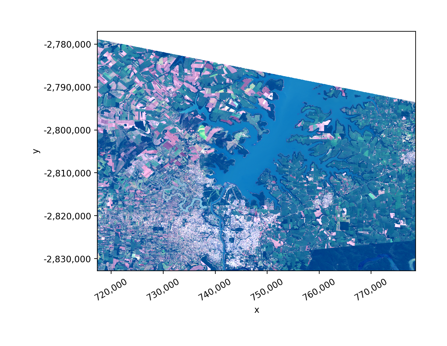
Open a raster as an xarray.DataArray.
In [10]: with gw.open(l8_224078_20200518) as src:
   ....:     print(src)
   ....:
<xarray.DataArray (band: 3, y: 1860, x: 2041)> Size: 23MB
dask.array<open_rasterio-6f781a4c543968cbbfe5469bb4a4f982<this-array>, shape=(3, 1860, 2041), dtype=uint16, chunksize=(3, 256, 256), chunktype=numpy.ndarray>
Coordinates:
  * band     (band) int64 24B 1 2 3
  * y        (y) float64 15kB -2.777e+06 -2.777e+06 ... -2.833e+06 -2.833e+06
  * x        (x) float64 16kB 7.174e+05 7.174e+05 ... 7.785e+05 7.786e+05
Attributes: (12/13)
    transform:           (30.0, 0.0, 717345.0, 0.0, -30.0, -2776995.0)
    crs:                 32621
    res:                 (30.0, 30.0)
    is_tiled:            1
    nodatavals:          (nan, nan, nan)
    _FillValue:          nan
    ...                  ...
    offsets:             (0.0, 0.0, 0.0)
    filename:            /home/docs/checkouts/readthedocs.org/user_builds/geo...
    resampling:          nearest
    AREA_OR_POINT:       Area
    _data_are_separate:  0
    _data_are_stacked:   0
Force the output data type.
In [11]: with gw.open(l8_224078_20200518, dtype='float64') as src:
   ....:     print(src.dtype)
   ....:
float64
Specify band names.
In [12]: with gw.open(l8_224078_20200518, band_names=['blue', 'green', 'red']) as src:
   ....:     print(src.band)
   ....:
<xarray.DataArray 'band' (band: 3)> Size: 60B
array(['blue', 'green', 'red'], dtype='<U5')
Coordinates:
  * band     (band) <U5 60B 'blue' 'green' 'red'
Use the sensor name to set band names.
In [13]: with gw.config.update(sensor='bgr'):
   ....:     with gw.open(l8_224078_20200518) as src:
   ....:         print(src.band)
   ....:
<xarray.DataArray 'band' (band: 3)> Size: 60B
array(['blue', 'green', 'red'], dtype='<U5')
Coordinates:
  * band     (band) <U5 60B 'blue' 'green' 'red'
To open multiple images stacked by bands, use a list of files with stack_dim='band'.
Open a list of files as an xarray.DataArray, with all bands stacked.
In [14]: with gw.open([l8_224078_20200518_B2, l8_224078_20200518_B3, l8_224078_20200518_B4],
   ....:              band_names=['b', 'g', 'r'],
   ....:              stack_dim='band') as src:
   ....:     print(src)
   ....:
<xarray.DataArray (band: 3, y: 1860, x: 2041)> Size: 23MB
dask.array<concatenate, shape=(3, 1860, 2041), dtype=uint16, chunksize=(1, 256, 256), chunktype=numpy.ndarray>
Coordinates:
  * band     (band) <U1 12B 'b' 'g' 'r'
  * y        (y) float64 15kB -2.777e+06 -2.777e+06 ... -2.833e+06 -2.833e+06
  * x        (x) float64 16kB 7.174e+05 7.174e+05 ... 7.785e+05 7.786e+05
Attributes: (12/13)
    transform:           (30.0, 0.0, 717345.0, 0.0, -30.0, -2776995.0)
    crs:                 32621
    res:                 (30.0, 30.0)
    is_tiled:            1
    nodatavals:          (nan,)
    _FillValue:          nan
    ...                  ...
    offsets:             (0.0,)
    filename:            ['LC08_L1TP_224078_20200518_20200518_01_RT_B2.TIF', ...
    resampling:          nearest
    AREA_OR_POINT:       Point
    _data_are_separate:  1
    _data_are_stacked:   1
To open multiple images as a time stack, change the input to a list of files.
Open a list of files as an xarray.DataArray.
In [15]: with gw.open([l8_224078_20200518, l8_224078_20200518],
   ....:              band_names=['blue', 'green', 'red'],
   ....:              time_names=['t1', 't2']) as src:
   ....:     print(src)
   ....:
<xarray.DataArray (time: 2, band: 3, y: 1860, x: 2041)> Size: 46MB
dask.array<concatenate, shape=(2, 3, 1860, 2041), dtype=uint16, chunksize=(1, 3, 256, 256), chunktype=numpy.ndarray>
Coordinates:
  * time     (time) <U2 16B 't1' 't2'
  * band     (band) <U5 60B 'blue' 'green' 'red'
  * y        (y) float64 15kB -2.777e+06 -2.777e+06 ... -2.833e+06 -2.833e+06
  * x        (x) float64 16kB 7.174e+05 7.174e+05 ... 7.785e+05 7.786e+05
Attributes: (12/13)
    transform:           (30.0, 0.0, 717345.0, 0.0, -30.0, -2776995.0)
    crs:                 32621
    res:                 (30.0, 30.0)
    is_tiled:            1
    nodatavals:          (nan, nan, nan)
    _FillValue:          nan
    ...                  ...
    offsets:             (0.0, 0.0, 0.0)
    filename:            ['LC08_L1TP_224078_20200518_20200518_01_RT.TIF', 'LC...
    resampling:          nearest
    AREA_OR_POINT:       Area
    _data_are_separate:  1
    _data_are_stacked:   1
Note
Xarray will handle alignment of images of varying sizes as long as the the resolutions are “target aligned”. If images are not target aligned, Xarray might not concatenate a stack of images. With GeoWombat, we can use a context manager and a reference image to handle image alignment.
In the example below, we specify a reference image using the geowombat configuration manager.
Note
The two images in this example are identical. The point here is just to illustrate the use of the configuration manager.
# Use an image as a reference for grid alignment and CRS-handling
#
# Within the configuration context, every image
# in concat_list will conform to the reference grid.
In [16]: filenames = [l8_224078_20200518, l8_224078_20200518]

In [17]: with gw.config.update(ref_image=l8_224077_20200518_B2):
   ....:     with gw.open(
   ....:         filenames,
   ....:         band_names=['blue', 'green', 'red'],
   ....:         time_names=['t1', 't2']
   ....:     ) as src:
   ....:         print(src)
   ....:
<xarray.DataArray (time: 2, band: 3, y: 1515, x: 2006)> Size: 36MB
dask.array<concatenate, shape=(2, 3, 1515, 2006), dtype=uint16, chunksize=(1, 3, 256, 256), chunktype=numpy.ndarray>
Coordinates:
  * time     (time) <U2 16B 't1' 't2'
  * band     (band) <U5 60B 'blue' 'green' 'red'
  * y        (y) float64 12kB -2.767e+06 -2.767e+06 ... -2.812e+06 -2.812e+06
  * x        (x) float64 16kB 6.94e+05 6.94e+05 ... 7.541e+05 7.542e+05
Attributes: (12/13)
    transform:           (30.0, 0.0, 694005.0, 0.0, -30.0, -2766615.0)
    crs:                 32621
    res:                 (30.0, 30.0)
    is_tiled:            1
    nodatavals:          (nan, nan, nan)
    _FillValue:          nan
    ...                  ...
    offsets:             (0.0, 0.0, 0.0)
    filename:            ['LC08_L1TP_224078_20200518_20200518_01_RT.TIF', 'LC...
    resampling:          nearest
    AREA_OR_POINT:       Area
    _data_are_separate:  1
    _data_are_stacked:   1

In [18]: with gw.config.update(ref_image=l8_224078_20200518_B2):
   ....:     with gw.open(
   ....:         filenames,
   ....:         band_names=['blue', 'green', 'red'],
   ....:         time_names=['t1', 't2']
   ....:     ) as src:
   ....:         print(src)
   ....:
<xarray.DataArray (time: 2, band: 3, y: 1860, x: 2041)> Size: 46MB
dask.array<concatenate, shape=(2, 3, 1860, 2041), dtype=uint16, chunksize=(1, 3, 256, 256), chunktype=numpy.ndarray>
Coordinates:
  * time     (time) <U2 16B 't1' 't2'
  * band     (band) <U5 60B 'blue' 'green' 'red'
  * y        (y) float64 15kB -2.777e+06 -2.777e+06 ... -2.833e+06 -2.833e+06
  * x        (x) float64 16kB 7.174e+05 7.174e+05 ... 7.785e+05 7.786e+05
Attributes: (12/13)
    transform:           (30.0, 0.0, 717345.0, 0.0, -30.0, -2776995.0)
    crs:                 32621
    res:                 (30.0, 30.0)
    is_tiled:            1
    nodatavals:          (nan, nan, nan)
    _FillValue:          nan
    ...                  ...
    offsets:             (0.0, 0.0, 0.0)
    filename:            ['LC08_L1TP_224078_20200518_20200518_01_RT.TIF', 'LC...
    resampling:          nearest
    AREA_OR_POINT:       Area
    _data_are_separate:  1
    _data_are_stacked:   1
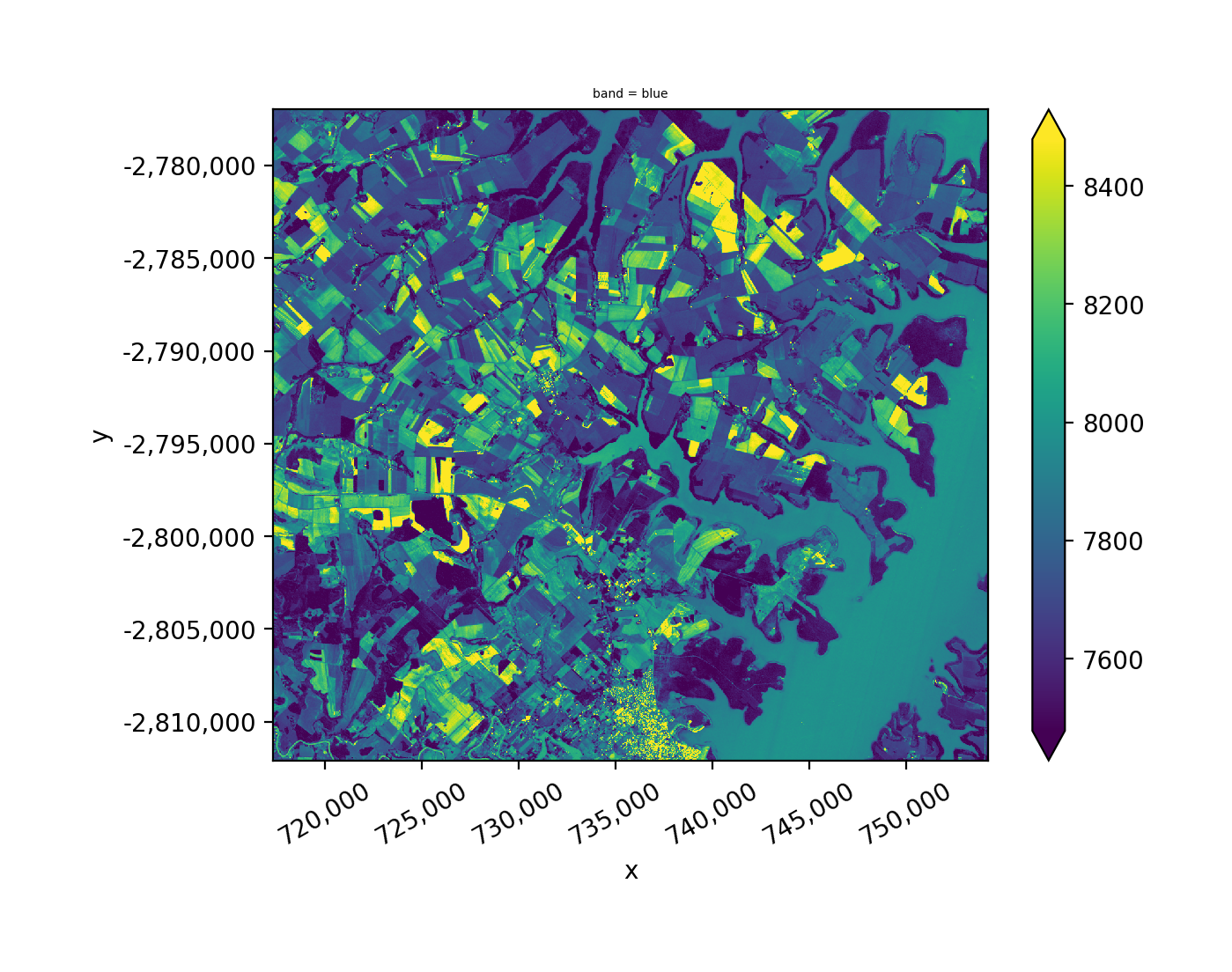
Stack the intersection of all images.
In [19]: fig, ax = plt.subplots(dpi=200)

In [20]: filenames = [l8_224077_20200518_B2, l8_224078_20200518_B2]

In [21]: with gw.open(
   ....:     filenames,
   ....:     band_names=['blue'],
   ....:     mosaic=True,
   ....:     bounds_by='intersection'
   ....: ) as src:
   ....:     src.where(src != 0).sel(band='blue').gw.imshow(robust=True, ax=ax)
   ....:

In [22]: plt.tight_layout(pad=1)
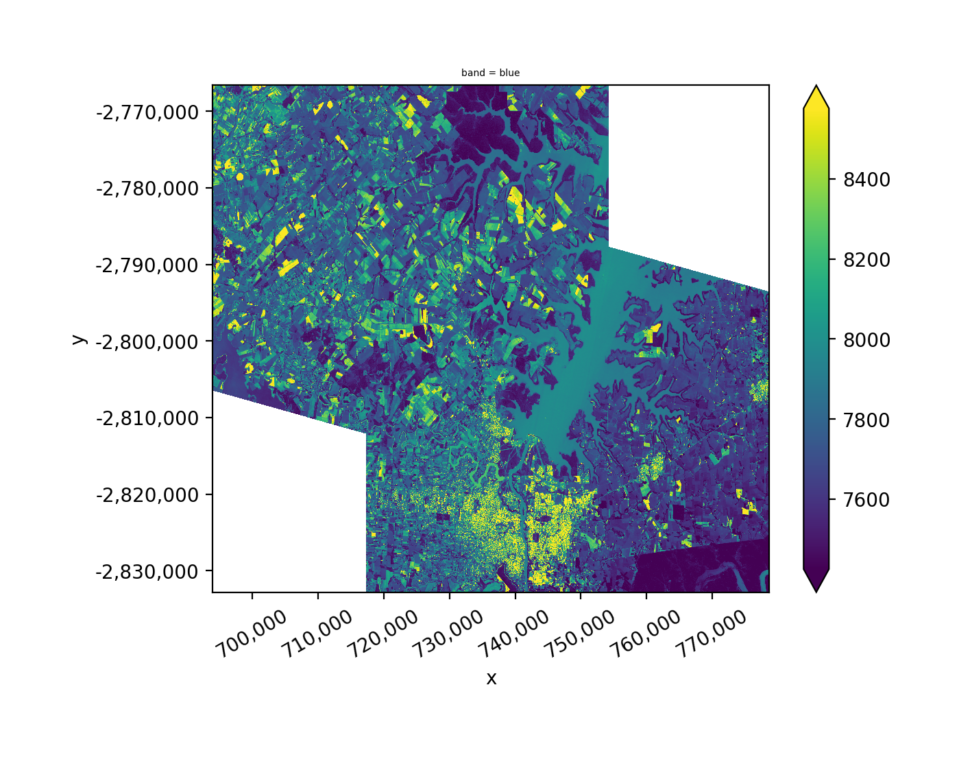
Stack the union of all images.
In [23]: fig, ax = plt.subplots(dpi=200)

In [24]: filenames = [l8_224077_20200518_B2, l8_224078_20200518_B2]

In [25]: with gw.open(
   ....:     filenames,
   ....:     band_names=['blue'],
   ....:     mosaic=True,
   ....:     bounds_by='union'
   ....: ) as src:
   ....:     src.where(src != 0).sel(band='blue').gw.imshow(robust=True, ax=ax)
   ....:

In [26]: plt.tight_layout(pad=1)
When multiple images have matching dates, the arrays are merged into one layer.
In [27]: filenames = [l8_224077_20200518_B2, l8_224078_20200518_B2]

In [28]: band_names = ['blue']

In [29]: time_names = ['t1', 't1']

In [30]: with gw.open(filenames, band_names=band_names, time_names=time_names) as src:
   ....:     print(src)
   ....:
<xarray.DataArray '_nanmax_skip-aggregate-34774903ffe0cbb71dc4be17d17f7d7b' (
                                                                             time: 1,
                                                                             band: 1,
                                                                             y: 1515,
                                                                             x: 2006)> Size: 24MB
dask.array<getitem, shape=(1, 1, 1515, 2006), dtype=float64, chunksize=(1, 1, 256, 256), chunktype=numpy.ndarray>
Coordinates:
  * time     (time) <U2 8B 't1'
  * band     (band) <U4 16B 'blue'
  * y        (y) float64 12kB -2.767e+06 -2.767e+06 ... -2.812e+06 -2.812e+06
  * x        (x) float64 16kB 6.94e+05 6.94e+05 ... 7.541e+05 7.542e+05
Attributes: (12/14)
    scales:              (1.0,)
    offsets:             (0.0,)
    nodatavals:          (nan,)
    _FillValue:          nan
    transform:           (30.0, 0.0, 694005.0, 0.0, -30.0, -2766615.0)
    crs:                 32621
    ...                  ...
    AREA_OR_POINT:       Point
    resampling:          nearest
    geometries:          [<POLYGON ((754185 -2812065, 754185 -2766615, 694005...
    filename:            ['LC08_L1TP_224077_20200518_20200518_01_RT_B2.TIF', ...
    _data_are_separate:  1
    _data_are_stacked:   1
Image mosaicking#
Mosaic the two subsets into a single xarray.DataArray. If the images in the mosaic list have the same CRS, no configuration
is needed.
In [31]: with gw.open(
   ....:     [l8_224077_20200518_B2, l8_224078_20200518_B2],
   ....:     band_names=['b'],
   ....:     mosaic=True
   ....: ) as src:
   ....:     print(src)
   ....:
<xarray.DataArray '_nanmax_skip-aggregate-34774903ffe0cbb71dc4be17d17f7d7b' (
                                                                             band: 1,
                                                                             y: 1515,
                                                                             x: 2006)> Size: 24MB
dask.array<where, shape=(1, 1515, 2006), dtype=float64, chunksize=(1, 256, 256), chunktype=numpy.ndarray>
Coordinates:
  * band     (band) <U1 4B 'b'
  * y        (y) float64 12kB -2.767e+06 -2.767e+06 ... -2.812e+06 -2.812e+06
  * x        (x) float64 16kB 6.94e+05 6.94e+05 ... 7.541e+05 7.542e+05
Attributes: (12/13)
    scales:              (1.0,)
    offsets:             (0.0,)
    nodatavals:          (nan,)
    _FillValue:          nan
    transform:           (30.0, 0.0, 694005.0, 0.0, -30.0, -2766615.0)
    crs:                 32621
    ...                  ...
    is_tiled:            1
    AREA_OR_POINT:       Point
    resampling:          nearest
    geometries:          [<POLYGON ((754185 -2812065, 754185 -2766615, 694005...
    _data_are_separate:  1
    _data_are_stacked:   0
If the images in the mosaic list have different CRSs, use a context manager to warp to a common grid.
Note
The two images in this example have the same CRS. The point here is just to illustrate the use of the configuration manager.
# Use a reference CRS
In [32]: with gw.config.update(ref_image=l8_224077_20200518_B2):
   ....:     with gw.open(
   ....:         [l8_224077_20200518_B2, l8_224078_20200518_B2],
   ....:         band_names=['b'],
   ....:         mosaic=True
   ....:     ) as src:
   ....:         print(src)
   ....:
<xarray.DataArray '_nanmax_skip-aggregate-34774903ffe0cbb71dc4be17d17f7d7b' (
                                                                             band: 1,
                                                                             y: 1515,
                                                                             x: 2006)> Size: 24MB
dask.array<where, shape=(1, 1515, 2006), dtype=float64, chunksize=(1, 256, 256), chunktype=numpy.ndarray>
Coordinates:
  * band     (band) <U1 4B 'b'
  * y        (y) float64 12kB -2.767e+06 -2.767e+06 ... -2.812e+06 -2.812e+06
  * x        (x) float64 16kB 6.94e+05 6.94e+05 ... 7.541e+05 7.542e+05
Attributes: (12/13)
    scales:              (1.0,)
    offsets:             (0.0,)
    nodatavals:          (nan,)
    _FillValue:          nan
    transform:           (30.0, 0.0, 694005.0, 0.0, -30.0, -2766615.0)
    crs:                 32621
    ...                  ...
    is_tiled:            1
    AREA_OR_POINT:       Point
    resampling:          nearest
    geometries:          [<POLYGON ((754185 -2812065, 754185 -2766615, 694005...
    _data_are_separate:  1
    _data_are_stacked:   0
Setup a plot function#
In [33]: def plot(bounds_by, ref_image=None, cmap='viridis'):
   ....:     fig, ax = plt.subplots(figsize=(10, 7), dpi=200)
   ....:     effective_bounds_by = 'reference' if ref_image is not None else bounds_by
   ....:     with gw.config.update(ref_image=ref_image):
   ....:         with gw.open(
   ....:             [l8_224077_20200518_B4, l8_224078_20200518_B4],
   ....:             band_names=['nir'],
   ....:             chunks=256,
   ....:             mosaic=True,
   ....:             bounds_by=effective_bounds_by,
   ....:             persist_filenames=True
   ....:         ) as srca:
   ....:             srca.where(srca != 0).sel(band='nir').gw.imshow(robust=True, cbar_kwargs={'label': 'DN'}, ax=ax)
   ....:             srca.gw.chunk_grid.plot(color='none', edgecolor='k', ls='-', lw=0.5, ax=ax)
   ....:             srca.gw.footprint_grid.plot(color='none', edgecolor='orange', lw=2, ax=ax)
   ....:             for row in srca.gw.footprint_grid.itertuples(index=False):
   ....:                 ax.scatter(
   ....:                     row.geometry.centroid.x,
   ....:                     row.geometry.centroid.y,
   ....:                     s=50, color='red', edgecolor='white', lw=1
   ....:                 )
   ....:                 ax.annotate(
   ....:                     row.footprint.replace('.TIF', ''),
   ....:                     (row.geometry.centroid.x, row.geometry.centroid.y),
   ....:                     color='black',
   ....:                     size=8,
   ....:                     ha='center',
   ....:                     va='center',
   ....:                     path_effects=[pe.withStroke(linewidth=1, foreground='white')]
   ....:                 )
   ....:             ax.set_ylim(
   ....:                 srca.gw.footprint_grid.total_bounds[1]-10,
   ....:                 srca.gw.footprint_grid.total_bounds[3]+10
   ....:             )
   ....:             ax.set_xlim(
   ....:                 srca.gw.footprint_grid.total_bounds[0]-10,
   ....:                 srca.gw.footprint_grid.total_bounds[2]+10
   ....:             )
   ....:     title = f'Image {bounds_by}' if bounds_by else str(Path(ref_image).name.split('.')[0]) + ' as reference'
   ....:     size = 12 if bounds_by else 8
   ....:     ax.set_title(title, size=size)
   ....:
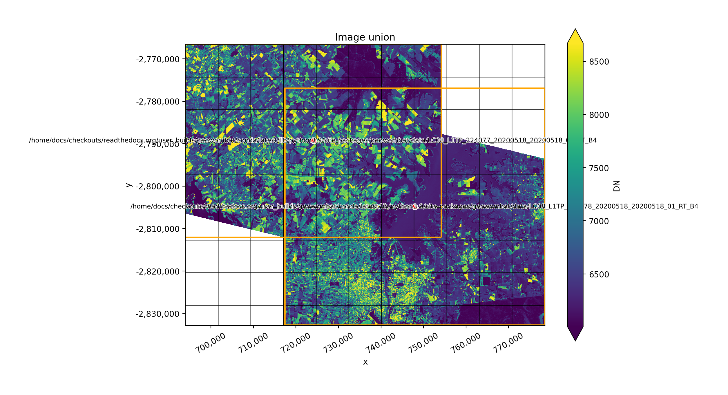
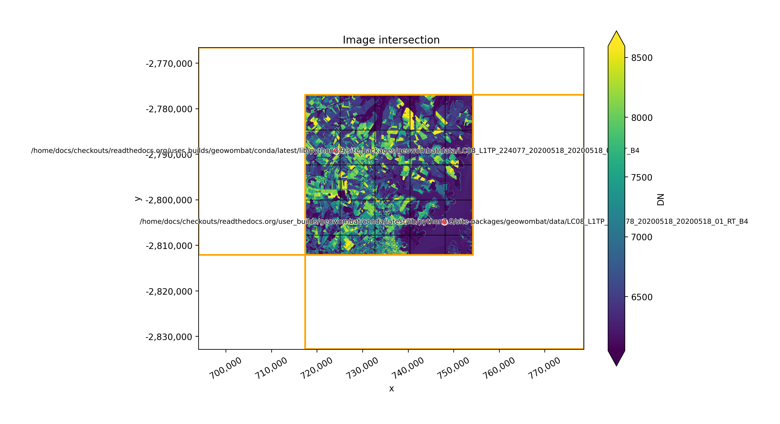
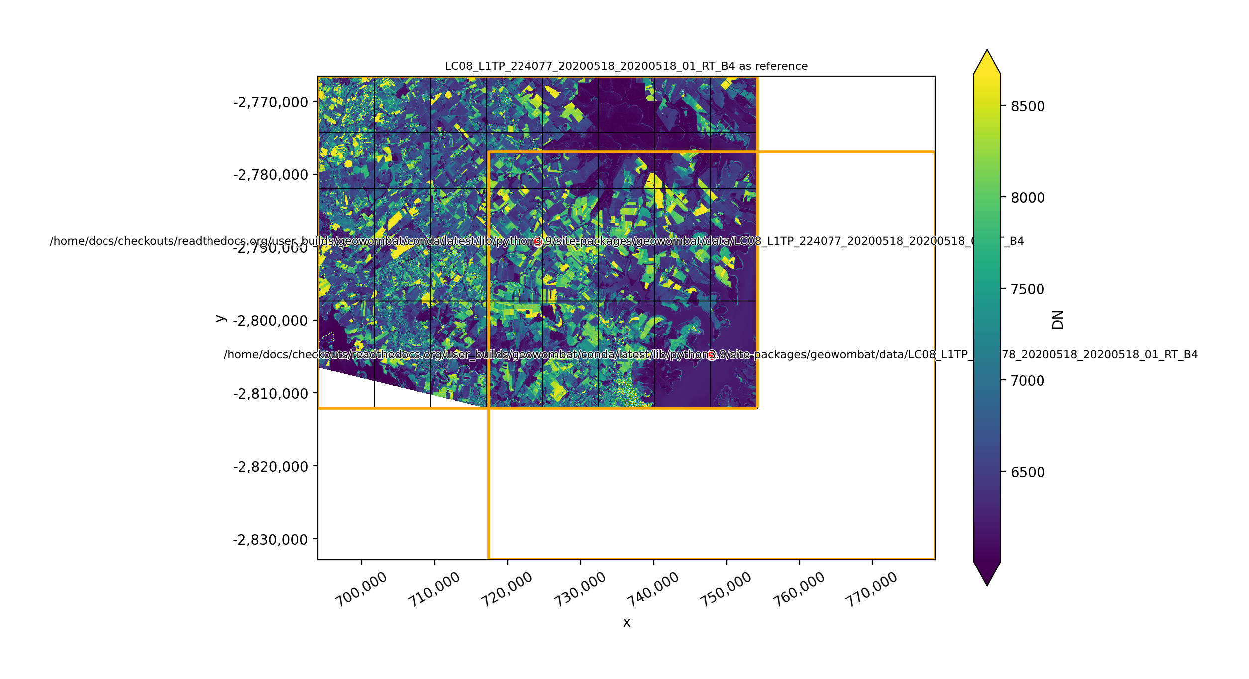
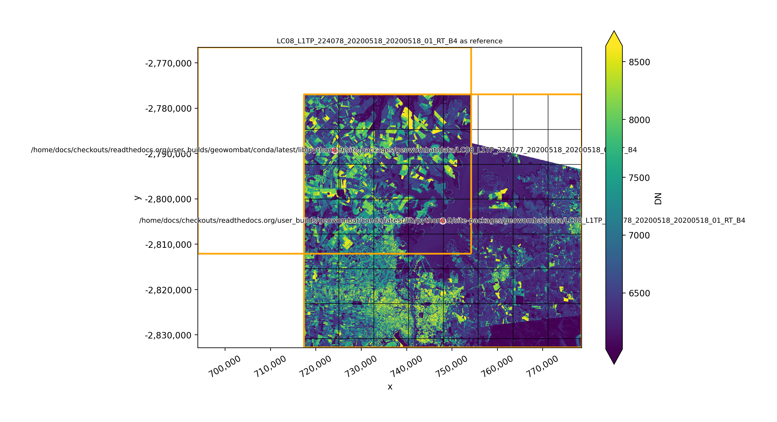
Mosaic by the union of images#
The two plots below illustrate how two images can be mosaicked. The orange grids highlight the image
footprints while the black grids illustrate the xarray.DataArray chunks.
In [34]: plot('union')
In [35]: plot('intersection')
In [36]: plot(None, l8_224077_20200518_B4)
In [37]: plot(None, l8_224078_20200518_B4)
Writing DataArrays to file#
GeoWombat’s file writing can be accessed through the geowombat to_vrt(), to_raster(),
and save() functions. These functions use rasterio.write() and Dask.array.store()
as I/O backends. In the examples below, src is an xarray.DataArray
with the necessary transform and coordinate reference system (CRS) information to write to an
image file.
Note
Should I use geowombat.to_raster() or geowombat.save() when writing a raster file? First, a bit of
background.
In the early days of geowombat development, direct computation calls using
dask (more on that with geowombat.save()) were tested on large raster files
(i.e., width and height on the order of tens of thousands). It was determined that the overhead
of generating the dask task graph was too large and outweighed the actual computation. To
address this, the geowombat.to_raster() method was designed to iterate over raster chunks/blocks
using concurrent.futures, reading and computing each block when requested. This removed
any large overhead but also negated the efficiency of dask as the underlying ‘delayed’
array. The geowombat.to_raster() can be used on data of any size, but comes with its own overhead.
For example, when working with arrays that fit into memory, such as a standard satellite scene,
dask (i.e., geowombat.save()) works quite well. To give an example, instead of slicing an xarray.DataArray
chunk and writing/computing that chunk (i.e., geowombat.to_raster() approach), we can also compute the entire
xarray.DataArray using dask (i.e., geowombat.save()) and let dask handle the concurrency. This is
where geowombat.save() comes in to play. The geowombat.save() method (or also xarray.DataArray.gw.save())
submits the data to Dask.array.store() and each chunk is written to file using rasterio.
The recommended method to use for saving raster files is geowombat.save(). We welcome feedback for
both methods, particularly if geowombat.save() is determined to be more efficient than geowombat.to_raster(),
regardless of the data size.
Write to a raster file using Dask and geowombat.save()#
import geowombat as gw

with gw.open(l8_224077_20200518_B4, chunks=1024) as src:
    # Xarray drops attributes
    attrs = src.attrs.copy()
    # Apply operations on the DataArray
    src = (src * 10.0).assign_attrs(**attrs)
    # Write the data to a GeoTiff
    src.gw.save(
        'output.tif',
        num_workers=4  # these workers are used as Dask.compute(num_workers=num_workers)
    )
Write to a raster file using concurrent.futures and geowombat.to_raster()#
import geowombat as gw

with gw.open(l8_224077_20200518_B4, chunks=1024) as src:
    # Xarray drops attributes
    attrs = src.attrs.copy()
    # Apply operations on the DataArray
    src = (src * 10.0).assign_attrs(**attrs)
    # Write the data to a GeoTiff
    src.gw.to_raster(
        'output.tif',
        verbose=1,
        n_workers=4,    # number of process workers sent to ``concurrent.futures``
        n_threads=2,    # number of thread workers sent to ``dask.compute``
        n_chunks=200    # number of window chunks to send as concurrent futures
    )
Write to a VRT file#
The GDAL VRT file format is a nice way to save data to file as a lightweight pointer to data on disk. A VRT file is an XML file that contains information about the image file, or files, needed to transform and display data (e.g., in a GIS).
Note
GeoWombat saves data to a VRT by re-opening the DataArray file or files (using
rasterio.vrt.WarpedVRT) and borrowing the DataArray attributes needed to correctly save
the data. Therefore, because we cannot currently pass a DataArray directly to the rasterio
VRT warper, any warping already applied using geowombat (e.g., with geowombat.config.update)
would be duplicated when writing the data to a VRT.
import geowombat as gw

# Transform the data to lat/lon
with gw.config.update(ref_crs=4326):
    with gw.open(l8_224077_20200518_B4, chunks=1024) as src:
        # Write the data to a VRT
        src.gw.to_vrt('lat_lon_file.vrt')
See Distributed processing for more examples describing concurrent file writing with GeoWombat.
Passing GDAL configuration options#
GeoWombat respects rasterio’s rasterio.Env context manager: any GDAL
configuration option can be set by wrapping a GeoWombat call inside rio.Env.
import rasterio as rio
import geowombat as gw

with rio.Env(GDAL_CACHEMAX=512, CPL_VSIL_CURL_USE_HEAD="NO"):
    with gw.open('image.tif') as src:
        src.gw.save('out.tif')
Multi-threaded warping is enabled by passing num_threads=N to gw.open,
gw.save, mosaic, concat, warp_open, or transform_crs.
Internally GeoWombat opens an inner rio.Env(GDAL_NUM_THREADS=str(N)) only
when num_threads > 1, which composes with any outer rio.Env. The
default num_threads=1 leaves the GDAL env untouched, so a user’s outer
rio.Env(GDAL_NUM_THREADS=...) flows through unmodified.
The threading sweet spot is workload-dependent. With dask-chunked reads
(chunks=...) the dask scheduler is already parallel across chunks, so
num_threads=2 is typically optimal and ALL_CPUS can over-subscribe the
machine. For eager or single-chunk reads, larger thread counts scale well.