Plotting raster data

# Import GeoWombat
In [1]: import geowombat as gw

# Load image names
In [2]: from geowombat.data import l8_224078_20200518, l8_224077_20200518_B2, l8_224078_20200518_B2

In [3]: from geowombat.data import l8_224077_20200518_B4, l8_224078_20200518_B4

In [4]: from pathlib import Path

In [5]: import matplotlib.pyplot as plt

In [6]: import matplotlib.patheffects as pe

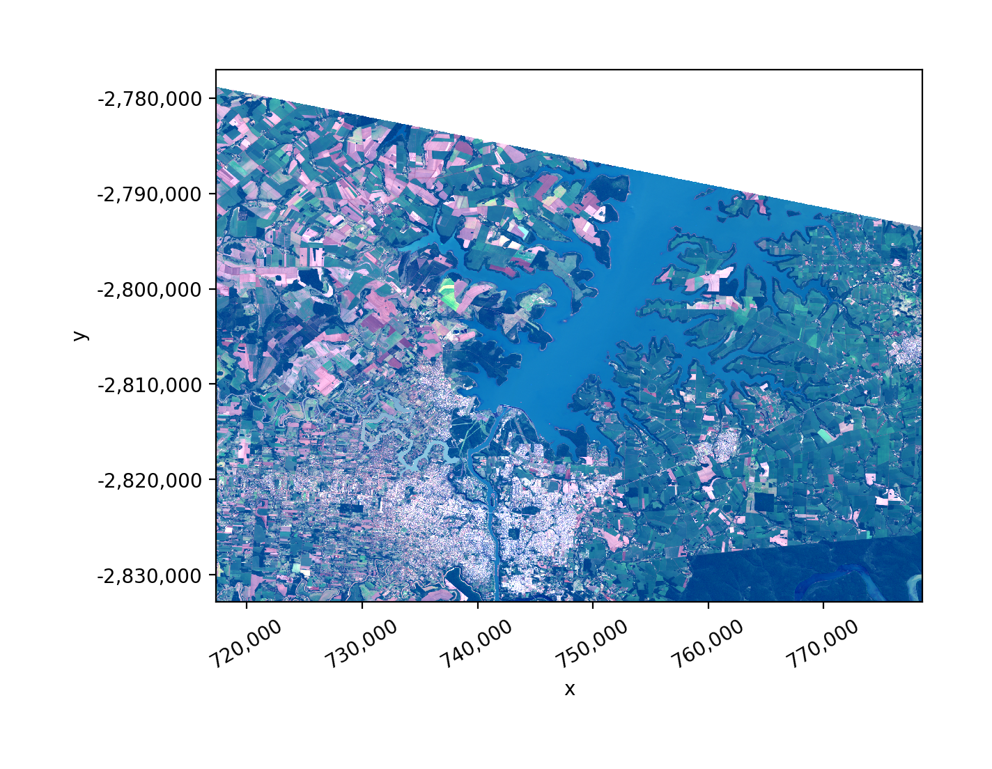
Plot the entire array

In [7]: fig, ax = plt.subplots(dpi=200)

In [8]: with gw.open(l8_224078_20200518) as src:
   ...:     src.where(src != 0).sel(band=[3, 2, 1]).gw.imshow(robust=True, ax=ax)
   ...: 

In [9]: plt.tight_layout(pad=1)

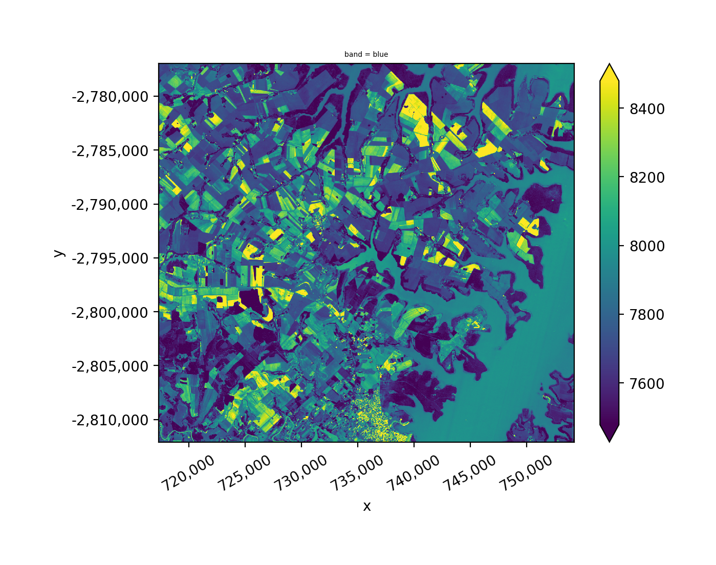
Plot the intersection of two arrays

In [10]: fig, ax = plt.subplots(dpi=200)

In [11]: filenames = [l8_224077_20200518_B2, l8_224078_20200518_B2]

In [12]: with gw.open(
   ....:     filenames,
   ....:     band_names=['blue'],
   ....:     mosaic=True,
   ....:     bounds_by='intersection'
   ....: ) as src:
   ....:     src.where(src != 0).sel(band='blue').gw.imshow(robust=True, ax=ax)
   ....: 

In [13]: plt.tight_layout(pad=1)

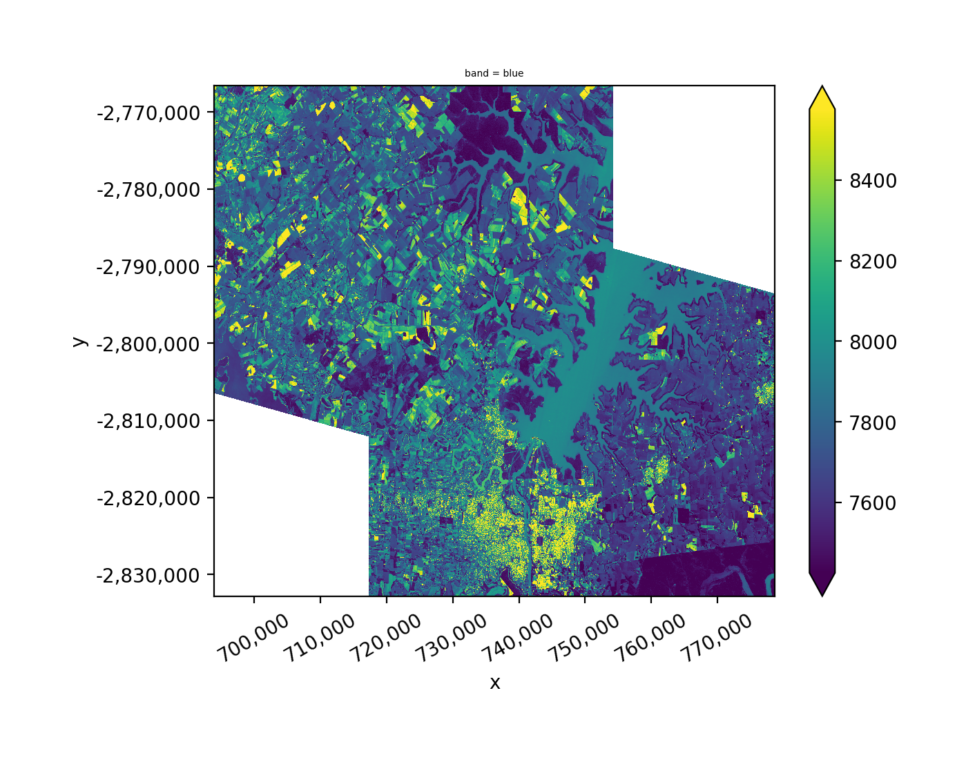
Plot the union of two arrays

In [14]: fig, ax = plt.subplots(dpi=200)

In [15]: filenames = [l8_224077_20200518_B2, l8_224078_20200518_B2]

In [16]: with gw.open(
   ....:     filenames,
   ....:     band_names=['blue'],
   ....:     mosaic=True,
   ....:     bounds_by='union'
   ....: ) as src:
   ....:     src.where(src != 0).sel(band='blue').gw.imshow(robust=True, ax=ax)
   ....: 

In [17]: plt.tight_layout(pad=1)

Setup a plot function

In [18]: def plot(bounds_by, ref_image=None, cmap='viridis'):
   ....:     fig, ax = plt.subplots(figsize=(10, 7), dpi=200)
   ....:     with gw.config.update(ref_image=ref_image):
   ....:         with gw.open(
   ....:             [l8_224077_20200518_B4, l8_224078_20200518_B4],
   ....:             band_names=['nir'],
   ....:             chunks=256,
   ....:             mosaic=True,
   ....:             bounds_by=bounds_by,
   ....:             persist_filenames=True
   ....:         ) as srca:
   ....:             srca.where(srca != 0).sel(band='nir').gw.imshow(robust=True, cbar_kwargs={'label': 'DN'}, ax=ax)
   ....:             srca.gw.chunk_grid.plot(color='none', edgecolor='k', ls='-', lw=0.5, ax=ax)
   ....:             srca.gw.footprint_grid.plot(color='none', edgecolor='orange', lw=2, ax=ax)
   ....:             for row in srca.gw.footprint_grid.itertuples(index=False):
   ....:                 ax.scatter(
   ....:                     row.geometry.centroid.x,
   ....:                     row.geometry.centroid.y,
   ....:                     s=50, color='red', edgecolor='white', lw=1
   ....:                 )
   ....:                 ax.annotate(
   ....:                     row.footprint.replace('.TIF', ''),
   ....:                     (row.geometry.centroid.x, row.geometry.centroid.y),
   ....:                     color='black',
   ....:                     size=8,
   ....:                     ha='center',
   ....:                     va='center',
   ....:                     path_effects=[pe.withStroke(linewidth=1, foreground='white')]
   ....:                 )
   ....:             ax.set_ylim(
   ....:                 srca.gw.footprint_grid.total_bounds[1]-10,
   ....:                 srca.gw.footprint_grid.total_bounds[3]+10
   ....:             )
   ....:             ax.set_xlim(
   ....:                 srca.gw.footprint_grid.total_bounds[0]-10,
   ....:                 srca.gw.footprint_grid.total_bounds[2]+10
   ....:             )
   ....:     title = f'Image {bounds_by}' if bounds_by else str(Path(ref_image).name.split('.')[0]) + ' as reference'
   ....:     size = 12 if bounds_by else 8
   ....:     ax.set_title(title, size=size)
   ....: 

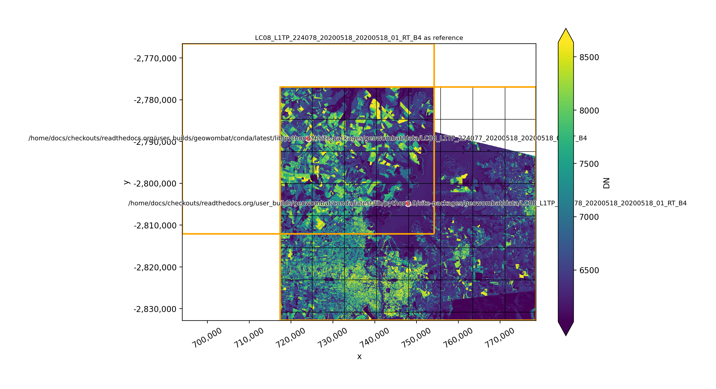
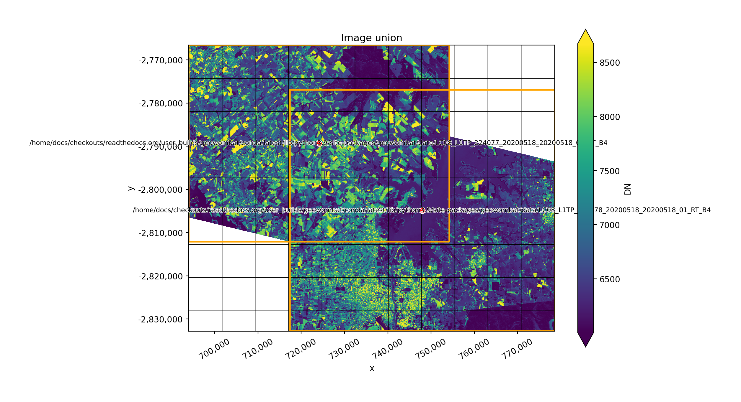
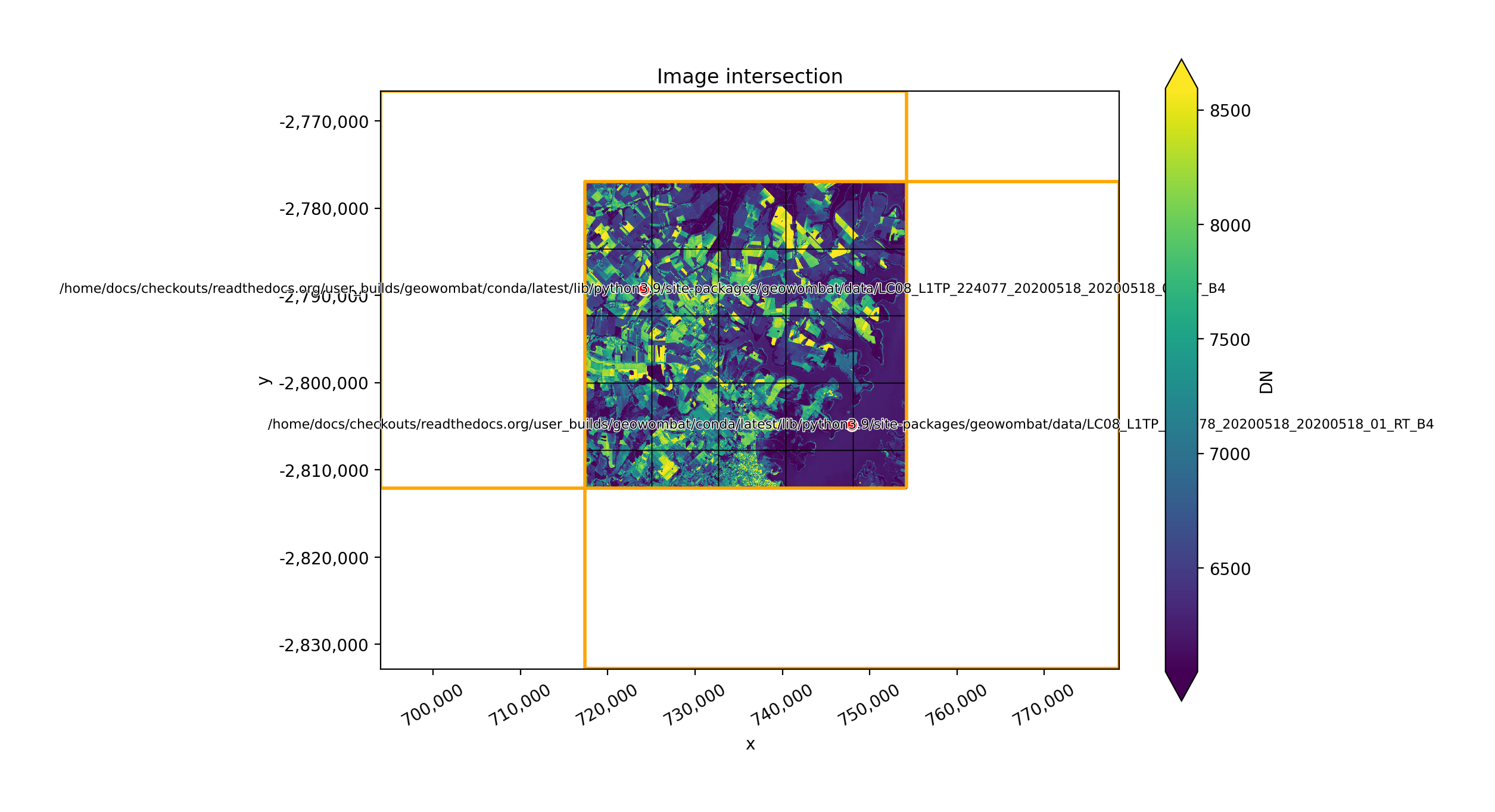
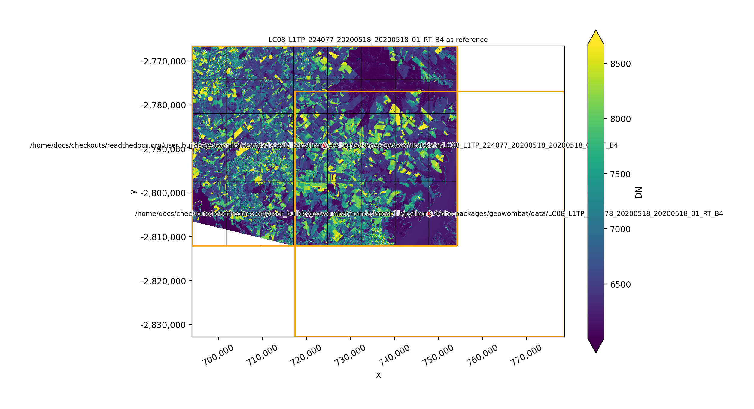
Image mosaics

The two plots below illustrate how two images can be mosaicked. The orange grids highlight the image footprints while the black grids illustrate the xarray.DataArray chunks.

In [19]: plot('union')

In [20]: plot('intersection')

In [21]: plot(None, l8_224077_20200518_B4)

In [22]: plot(None, l8_224078_20200518_B4)