Deep learning classifiers#

GeoWombat provides deep learning classifiers that follow the same fit() / predict() / fit_predict() API as the sklearn-based classifiers in the Machine learning module. Three architectures are included:

Classifier	Architecture	Best for
`TabNetClassifier`	Attention-based tabular model	Pixel-wise classification from spectral bands (single or multi-date)
`LTAEClassifier`	Lightweight Temporal Attention Encoder	Satellite image time series (requires `time` dimension)
`TorchGeoClassifier`	U-Net, DeepLabV3+, FPN segmentation	Spatial-context classification with optional pre-trained encoders

Setup and installation#

Install the deep learning dependencies:

pip install "geowombat[dl]"

This installs:

PyTorch (torch>=2.0.0)
pytorch-tabnet (pytorch-tabnet>=4.0)
TorchGeo (torchgeo>=0.6.0)
segmentation-models-pytorch (segmentation-models-pytorch>=0.3.0)

GPU setup#

By default, classifiers run on CPU. To use a GPU, you need a CUDA-enabled PyTorch installation. The easiest way is to follow the official PyTorch Get Started page — select your OS, package manager, and CUDA version to get the correct install command.

For example, with pip and CUDA 12.4:

pip install torch --index-url https://download.pytorch.org/whl/cu124

To verify your GPU is available:

import torch
print(torch.cuda.is_available())   # True if GPU is ready
print(torch.cuda.device_count())   # Number of GPUs
print(torch.cuda.get_device_name(0))  # GPU name

Then pass device='cuda' or device='auto' to any DL classifier:

TabNetClassifier(device='cuda')
LTAEClassifier(device='auto')      # auto-selects GPU if available
TorchGeoClassifier(device='cuda')

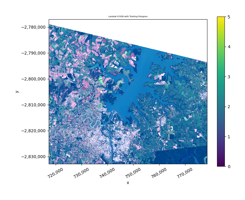
Prepare training labels#

All examples below use the bundled Landsat 8 test image and training polygons.

import warnings
warnings.filterwarnings('ignore')

import matplotlib.pyplot as plt
import geopandas as gpd
import numpy as np

import geowombat as gw
from geowombat.data import l8_224078_20200518, stac_training
from geowombat.ml import fit, fit_predict, predict

# Load training polygons (integer 'lc' column, EPSG:4326)
labels = gpd.read_file(stac_training)
print(f"Classes: {sorted(labels['lc'].unique())}")
print(f"Number of classes: {labels['lc'].nunique()}")

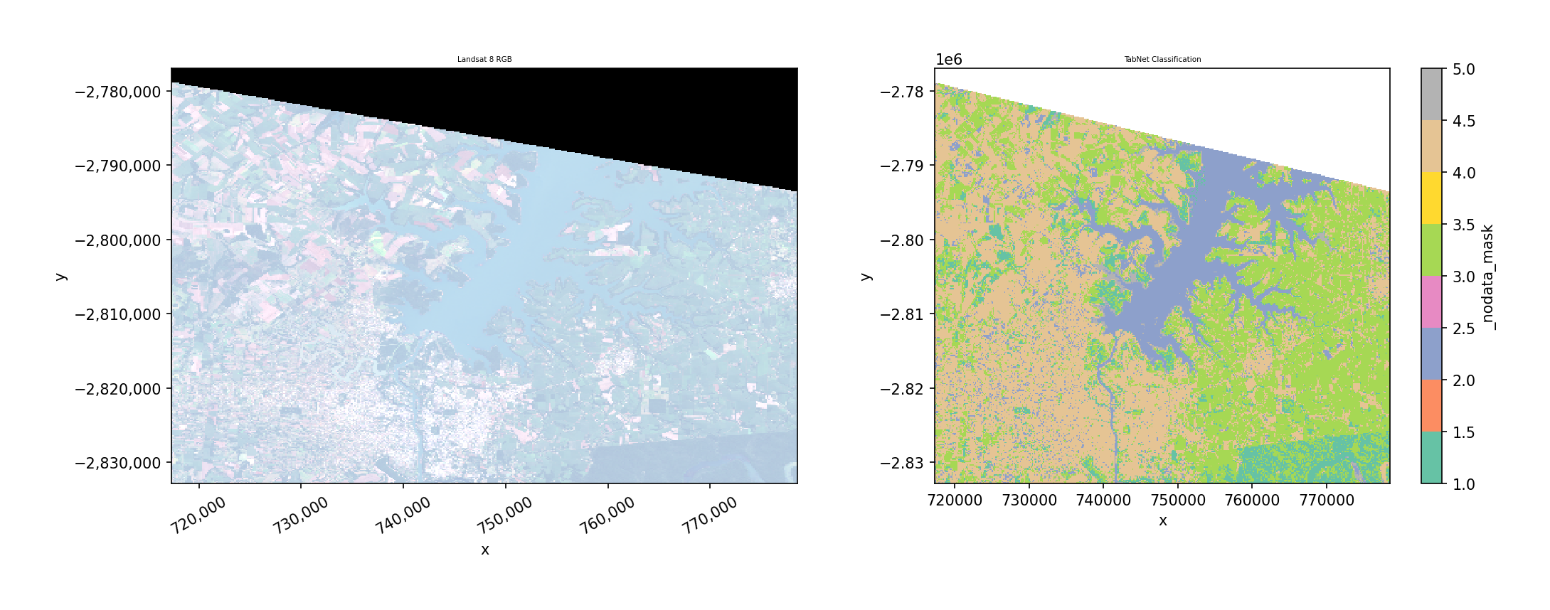
TabNet#

TabNet is an attention-based model for tabular data. Each pixel is treated as a sample with spectral bands as features. It works on single-date or multi-date imagery (bands are flattened to features).

n_classes is automatically inferred from the label column — you never need to specify it. Features are standardized internally before training.

Key parameters:

max_epochs: Training epochs (default 50)
batch_size: Mini-batch size (default 1024)
patience: Early stopping patience (default 10)
device: 'cpu', 'cuda', or 'auto'
verbose: 0 = silent, 1 = progress

fit_predict (one step)#

from geowombat.ml.dl_classifiers import TabNetClassifier

with gw.config.update(ref_res=150):
    with gw.open(l8_224078_20200518, nodata=0) as src:
        y = fit_predict(
            src,
            TabNetClassifier(max_epochs=50, verbose=0),
            labels,
            col='lc',
        )

print(y.shape)   # (1, 372, 408)
print(y.dims)    # ('band', 'y', 'x')

TabNet: separate fit then predict#

Use separate steps when you want to inspect the trained model, save it, or predict on different data.

with gw.config.update(ref_res=150):
    with gw.open(l8_224078_20200518, nodata=0) as src:
        clf = TabNetClassifier(max_epochs=50, verbose=0)

        # Step 1: fit
        X, Xy, clf = fit(src, clf, labels, col='lc')
        print(clf.fitted_)      # True
        print(clf._n_classes)   # 4

        # Step 2: predict
        y = predict(src, X, clf)

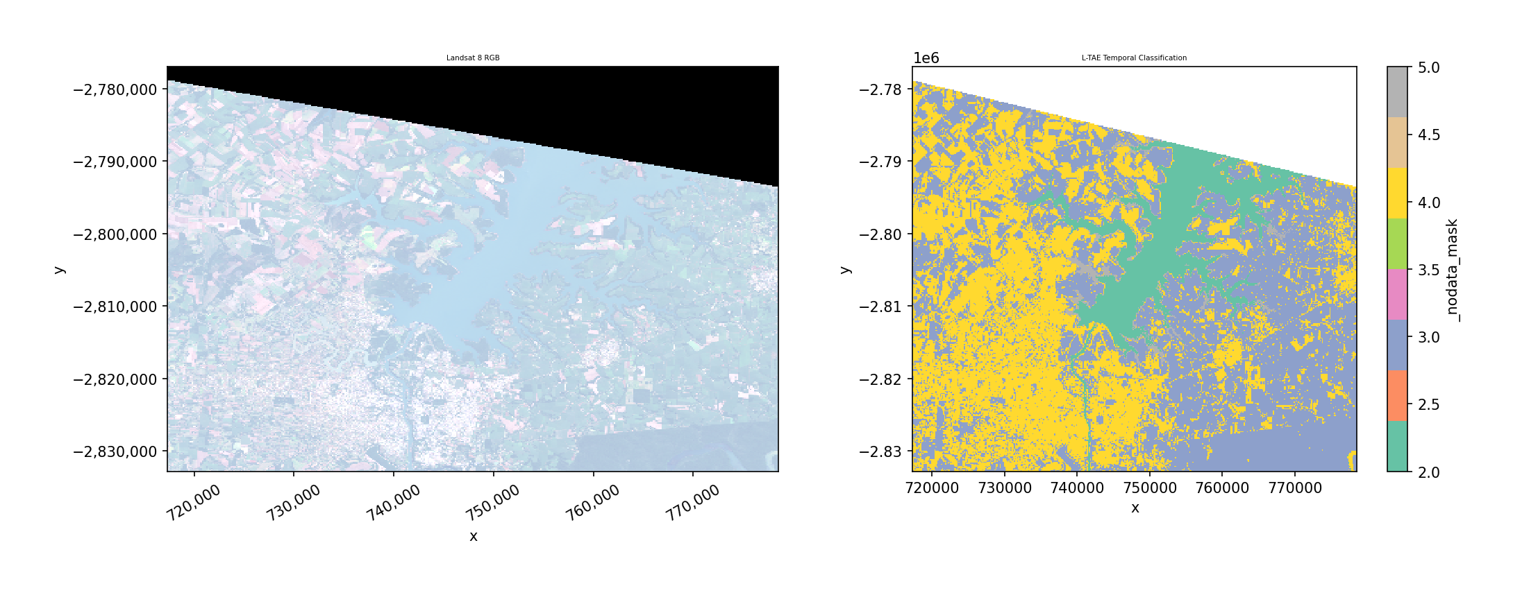
L-TAE (Temporal Attention)#

The Lightweight Temporal Attention Encoder (L-TAE) classifies pixels based on their spectral trajectory across multiple dates. It uses multi-head temporal attention with a learned master query.

Requires multi-temporal data with a time dimension (open with stack_dim='time'). Raises ValueError if data has no time dimension.

Key parameters:

n_head: Attention heads (default 4)
d_k: Key dimension per head (default 32)
d_model: Embedding dimension (default 128)
max_epochs: Training epochs (default 50)
lr: Learning rate (default 1e-3)
device: 'cpu', 'cuda', or 'auto'

fit_predict with time-stacked data#

from geowombat.ml.dl_classifiers import LTAEClassifier

with gw.config.update(ref_res=150):
    with gw.open(
        [l8_224078_20200518, l8_224078_20200518],
        stack_dim='time',
        nodata=0,
    ) as src:
        print(src.shape)  # (2, 3, 372, 408)
        print(src.dims)   # ('time', 'band', 'y', 'x')

        y = fit_predict(
            src,
            LTAEClassifier(
                max_epochs=50, verbose=0,
                d_model=32, d_k=8, n_head=2,
            ),
            labels,
            col='lc',
        )

Note

This demo stacks the same image twice. In practice, use imagery from different acquisition dates — L-TAE is most useful when temporal patterns differ between classes (e.g., crop phenology vs. forest).

L-TAE: separate fit then predict#

with gw.config.update(ref_res=150):
    with gw.open(
        [l8_224078_20200518, l8_224078_20200518],
        stack_dim='time',
        nodata=0,
    ) as src:
        clf = LTAEClassifier(
            max_epochs=50, verbose=0,
            d_model=32, d_k=8, n_head=2,
        )
        X, Xy, clf = fit(src, clf, labels, col='lc')
        y = predict(src, X, clf)

Error without time dimension#

L-TAE raises a clear error if the data is missing the time dimension:

with gw.open(l8_224078_20200518, nodata=0) as src:
    clf = LTAEClassifier()
    fit(src, clf, labels, col='lc')
# ValueError: LTAEClassifier requires multi-temporal data
# with a 'time' dimension. Open data with stack_dim='time'.

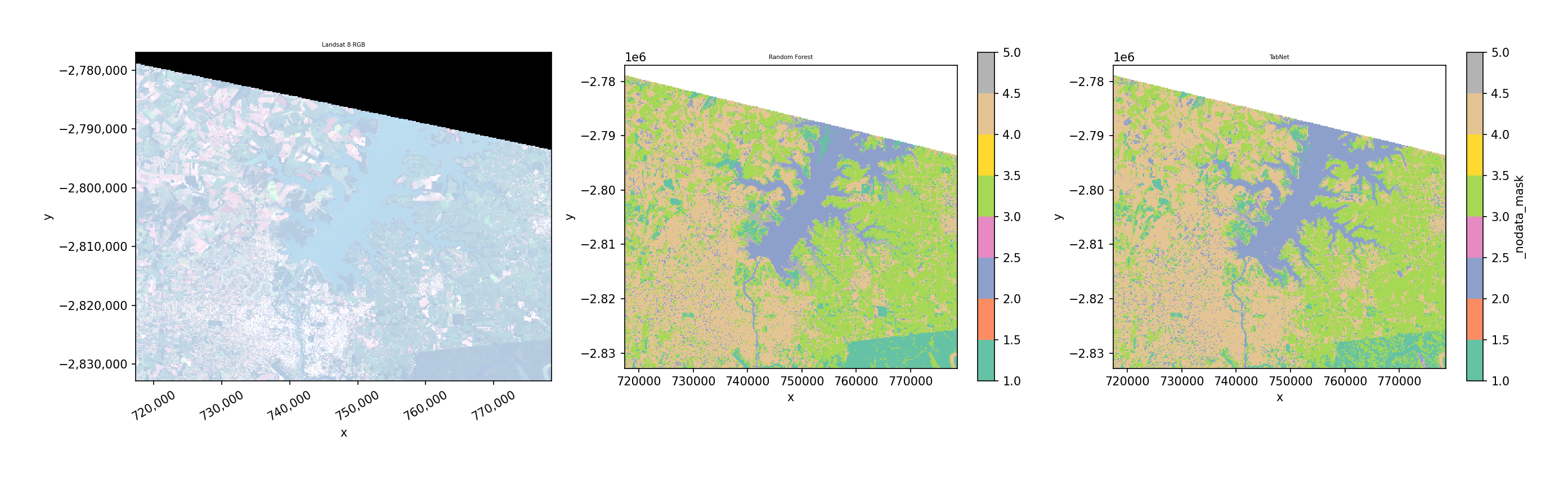
Comparison with sklearn classifiers#

The DL classifiers use the exact same API as sklearn classifiers — just swap the classifier object:

from sklearn.ensemble import RandomForestClassifier

with gw.config.update(ref_res=150):
    with gw.open(l8_224078_20200518, nodata=0) as src:
        # sklearn
        y_rf = fit_predict(
            src, RandomForestClassifier(n_estimators=50),
            labels, col='lc',
        )
        # DL
        y_tabnet = fit_predict(
            src, TabNetClassifier(max_epochs=50, verbose=0),
            labels, col='lc',
        )

TorchGeo segmentation models#

TorchGeoClassifier wraps segmentation models from segmentation-models-pytorch with optional pre-trained encoder weights from TorchGeo. It uses patch-based training and sliding-window inference.

Supported models: unet, deeplabv3+, deeplabv3, fcn (FPN).

Key parameters:

model: Model architecture (default 'unet')
backbone: Encoder backbone (default 'resnet18')
weights: TorchGeo weight name or None for random init
patch_size: Training/inference patch size (default 64)
stride: Inference stride (default patch_size // 2)
max_patches: Max training patches (default 500)
bands: Band indices or names to select (optional)
max_epochs, batch_size, lr, device

U-Net example#

from geowombat.ml.dl_classifiers import TorchGeoClassifier

with gw.config.update(ref_res=300):
    with gw.open(l8_224078_20200518, nodata=0) as src:
        clf = TorchGeoClassifier(
            model='unet',
            backbone='resnet18',
            weights=None,          # random init for demo
            patch_size=16,
            max_patches=20,
            max_epochs=2,
            batch_size=4,
            verbose=0,
        )
        y = fit_predict(src, clf, labels, col='lc')

Pre-trained encoder weights#

TorchGeo provides encoder weights pre-trained on satellite imagery (Sentinel-2, Landsat, NAIP). For a complete list of all available weights and their required inputs, see the TorchGeo pretrained weights reference.

Use the weights parameter and bands to match the model’s expected input:

# Sentinel-2 RGB pre-trained encoder
clf = TorchGeoClassifier(
    model='unet',
    backbone='resnet18',
    weights='ResNet18_Weights.SENTINEL2_RGB_MOCO',
    bands=[1, 2, 3],        # select bands matching model
    patch_size=64,
)

# Check what bands the model expects
print(clf.expected_bands)
# {'in_chans': 3, 'meta': {...}}

If the number of input bands doesn’t match the model’s expectations, a clear error is raised with guidance on how to fix it.

Available pretrained weights#

The table below summarizes the most common TorchGeo pretrained weight families. See the notebooks/dl_classifiers.ipynb notebook for an interactive table of all 60+ weights generated programmatically.

Sensor	Bands	Example Weight	Backbones
Sentinel-2 RGB	3	`SENTINEL2_RGB_MOCO`	ResNet18, ResNet50
Sentinel-2 All	13	`SENTINEL2_ALL_MOCO`	ResNet18, ResNet50, ViTSmall16
Sentinel-2 MS	9	`SENTINEL2_MI_MS_SATLAS`	ResNet50, Swin_V2_B
Landsat TM	7	`LANDSAT_TM_TOA_MOCO`	ResNet18, ResNet50
Landsat OLI SR	7	`LANDSAT_OLI_SR_MOCO`	ResNet18, ResNet50
Landsat OLI+TIRS	11	`LANDSAT_OLI_TIRS_TOA_MOCO`	ResNet18, ResNet50
Sentinel-1 SAR	2	`SENTINEL1_GRD_MOCO`	ResNet50
NAIP RGB	3	`NAIP_RGB_MI_SATLAS`	Swin_V2_B
fMoW RGB	3	`FMOW_RGB_GASSL`	ResNet50

To use a weight, pass it as weights='<BackboneName>_Weights.<WEIGHT_NAME>'. For example:

TorchGeoClassifier(
    backbone='resnet18',
    weights='ResNet18_Weights.SENTINEL2_RGB_MOCO',
    bands=[1, 2, 3],
)

see the TorchGeo pretrained weights reference for more details.

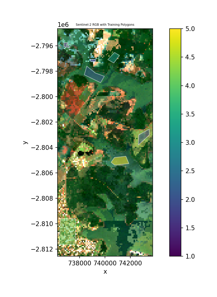
STAC + pretrained model example#

Download Sentinel-2 imagery from a STAC catalog and classify it using a pretrained TorchGeo encoder. composite_stac() creates a cloud-free median composite with automatic cloud masking via the Sentinel-2 SCL band.

from geowombat.core.stac import composite_stac
from geowombat.ml.dl_classifiers import TorchGeoClassifier

# Cloud-free yearly median composite
data, metadata = composite_stac(
    stac_catalog="element84_v1",
    collection="sentinel_s2_l2a",
    bounds=(-54.65, -25.41, -54.58, -25.25),
    epsg=32621,
    bands=["red", "green", "blue"],
    start_date="2023-01-01",
    end_date="2023-12-31",
    cloud_cover_perc=30,
    resolution=100.0,
    frequency="YS",       # yearly composite
    agg="median",
    max_items=20,
    compute=True,
)
img = data.isel(time=0)

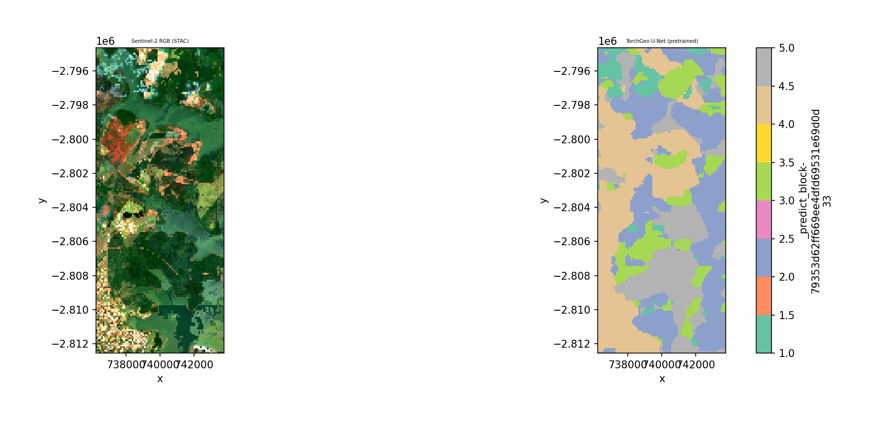
Sentinel-2 RGB composite with training polygons

Classify the composite with a U-Net using a Sentinel-2 RGB pretrained encoder:

clf = TorchGeoClassifier(
    model='unet',
    backbone='resnet18',
    weights='ResNet18_Weights.SENTINEL2_RGB_MOCO',
    patch_size=32,
    max_epochs=5,
    batch_size=4,
    verbose=0,
)
y = fit_predict(img, clf, labels, col='lc')

TorchGeo pretrained U-Net classification of STAC imagery

Note

composite_stac() requires network access and pip install geowombat[stac]. See the notebooks/dl_classifiers.ipynb notebook for a runnable version with error handling for offline use.

Notes#

n_classes is auto-inferred from the label column during fit(). You never need to specify it.
Feature normalization is handled internally — raw DN values are standardized before training and prediction.
Labels use 1-based encoding internally (0 = nodata). The classifiers convert to 0-based for PyTorch and back automatically.
Device: Pass device='cuda' or device='auto' for GPU acceleration.
For production workflows, increase max_epochs (e.g., 50–200) and use full-resolution data with more training samples.

Save predictions#

y.gw.save('classification.tif', overwrite=True)

Object detection#

In addition to pixel/patch classification, geowombat ships object detectors (axis-aligned and oriented bounding boxes) that return georeferenced GeoDataFrame outputs. They live in a dedicated geowombat.detect module and follow the same with gw.open(...) as src: / src.gw.<method>(...) shape as the rest of geowombat, with module-level wrappers in gw.detect that mirror gw.ml.fit / predict / fit_predict.

See Object detection for the full walkthrough.

Detector classes

geowombat.detect.YOLODetector — Ultralytics YOLO (AGPL-3.0). Requires pip install geowombat[detect].
geowombat.detect.TorchGeoDetector — Faster R-CNN / RetinaNet via TorchVision + optional TorchGeo weights. Already covered by geowombat[dl].
geowombat.detect.SAMRefiner — refine boxes to polygon masks with Segment Anything. Requires pip install geowombat[sam].

``.gw`` accessor and module-level entry points

src.gw.detect(detector, ...) — run tiled inference; returns a GeoDataFrame in the source CRS.
src.gw.to_yolo_dataset(labels, class_col=..., out_dir=...) — tile the raster + labels into an Ultralytics-layout dataset on disk.
gw.detect.predict(src, detector, ...) — module-level form of the accessor (parallels gw.ml.predict).
gw.detect.fit(detector, dataset_yaml, ...) — fine-tune a detector on a YOLO dataset.
gw.detect.fit_predict(src, detector, labels, class_col, out_dir, ...) — build → fine-tune → predict in one call.
gw.detect.build_dataset(...) — function form of .gw.to_yolo_dataset (alias for build_yolo_dataset).

Accuracy and review

gw.detect.boxes_from_polygons — convert polygon labels to axis-aligned or oriented boxes.
gw.detect.detection_accuracy — per-class precision / recall / F1 / AP at one or more IoU thresholds, with a review-ready GeoDataFrame.
gw.detect.export_for_review / recompute_from_review — write a GeoPackage you can step through in QGIS (e.g. with the GoToNextFeature3+ plugin), and recompute metrics after a human has filled in the reviewer_label field.

Quick example#

import geopandas as gpd
import geowombat as gw
from geowombat.detect import YOLODetector, detection_accuracy

buildings = gpd.read_file('buildings.gpkg')

with gw.config.update(sensor='rgb'):
    with gw.open('naip.tif', chunks=512) as src:

        # 1. Tile the raster + labels into a YOLO dataset
        src.gw.to_yolo_dataset(
            buildings, class_col='class_name',
            out_dir='./yolo', tile_size=640,
        )

        # 2. Run inference with a pre-built detector
        det = YOLODetector(weights='yolov8n.pt')
        preds = src.gw.detect(det, conf=0.1)

# 3. Score the predictions
results = detection_accuracy(
    preds, buildings, class_col='class_name',
    iou_thresholds=(0.3, 0.5),
)
print(results['summary'])

When gw.config.update(sensor=...) sets named bands (e.g. sensor='rgb' or sensor='bgr'), src.gw.detect and src.gw.to_yolo_dataset derive the RGB band indices from the active config; you don’t need to pass band_indices per call. Explicit band_indices=[...] still wins.

See the notebooks/object_detection.ipynb notebook for an end-to-end walkthrough using NAIP aerial imagery plus OpenStreetMap building footprints.

Deep learning classifiers

Contents

Deep learning classifiers#

Setup and installation#

GPU setup#

Prepare training labels#

TabNet#

fit_predict (one step)#

TabNet: separate fit then predict#

L-TAE (Temporal Attention)#

fit_predict with time-stacked data#

L-TAE: separate fit then predict#

Error without time dimension#

Comparison with sklearn classifiers#

TorchGeo segmentation models#

U-Net example#

Pre-trained encoder weights#

Available pretrained weights#

STAC + pretrained model example#

Notes#

Save predictions#

Object detection#

Quick example#