Machine Learning Classification in GeoWombat#

This notebook demonstrates machine learning classification for remote sensing data using geowombat and scikit-learn. It covers:

Supervised classification (fit/predict and fit_predict)
Unsupervised classification (KMeans)
Time series stacking with stack_dim='band'
Cross-validation & hyperparameter tuning
Time-dimensioned data with temporal_mode='panel' and temporal_mode='flatten'

Requirements: pip install geowombat[ml]

Based on the pygis tutorial.

Setup#

[21]:

import os
os.environ['CPL_LOG'] = '/dev/null'  # suppress GDAL warnings

import warnings

import geopandas as gpd
import matplotlib.pyplot as plt
import numpy as np
from sklearn.cluster import KMeans
from sklearn.decomposition import PCA
from sklearn.ensemble import RandomForestClassifier
from sklearn.naive_bayes import GaussianNB
from sklearn.pipeline import Pipeline
from sklearn.preprocessing import LabelEncoder, StandardScaler

import geowombat as gw
from geowombat.data import (
    l8_224078_20200518,
    l8_224078_20200518_points,
    stac_training,
)
from geowombat.ml import fit, fit_predict, predict

warnings.filterwarnings('ignore', category=(DeprecationWarning))
warnings.filterwarnings('ignore', category=(FutureWarning))
warnings.filterwarnings('ignore', category=(UserWarning))

Load training data#

We use labeled polygons and points bundled with geowombat. The polygon labels in stac_training have an integer lc column. The point labels use string class names that we encode with LabelEncoder.

[22]:

# Polygon labels (integer 'lc' column, EPSG:4326)
labels_poly = gpd.read_file(stac_training)
print('Polygon labels:')
print(f"  CRS: {labels_poly.crs}")
print(f"  Classes: {sorted(labels_poly['lc'].unique())}")
print(labels_poly[['lc', 'geometry']].head())

# Point labels (need LabelEncoder for string names)
le = LabelEncoder()
labels_point = gpd.read_file(l8_224078_20200518_points)
labels_point['lc'] = le.fit(labels_point.name).transform(labels_point.name)
labels_point = labels_point.drop(columns=['name'])
print('\nPoint labels:')
print(labels_point.head())

Polygon labels:
  CRS: EPSG:4326
  Classes: [0, 1, 2, 3, 5]
   lc                                           geometry
0   0  POLYGON ((-54.64919 -25.25946, -54.64925 -25.2...
1   0  POLYGON ((-54.62817 -25.27092, -54.62803 -25.2...
2   2  POLYGON ((-54.6147 -25.27095, -54.60949 -25.26...
3   1  POLYGON ((-54.61715 -25.28278, -54.62002 -25.2...
4   1  POLYGON ((-54.58943 -25.32398, -54.58966 -25.3...

Point labels:
                          geometry  lc
0  POINT (741522.314 -2811204.698)   3
1  POINT (736140.845 -2806478.364)   0
2  POINT (745919.508 -2805168.579)   2
3  POINT (739056.735 -2811710.662)   1
4  POINT (737802.183 -2818016.412)   3

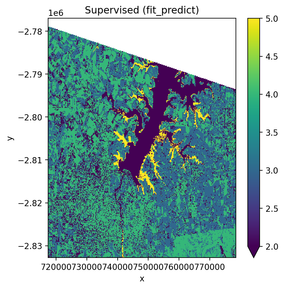
1. Supervised Classification#

Build a sklearn Pipeline with StandardScaler → PCA → GaussianNB, then train and predict on a Landsat 8 image.

Using `fit()` then `predict()` (two-step)#

[23]:

pl = Pipeline(
    [
        ('scaler', StandardScaler()),
        ('pca', PCA()),
        ('clf', GaussianNB()),
    ]
)

fig, ax = plt.subplots(dpi=200, figsize=(5, 5))

with gw.config.update(ref_res=150):
    with gw.open(l8_224078_20200518, nodata=0) as src:
        X, Xy, clf = fit(src, pl, labels_poly, col='lc')
        y = predict(src, X, clf)
        y.plot(robust=True, ax=ax)

ax.set_title('Supervised (fit + predict)')
plt.tight_layout(pad=1)
plt.show()

Using `fit_predict()` (one-step)#

[24]:

fig, ax = plt.subplots(dpi=200, figsize=(5, 5))

with gw.config.update(ref_res=150):
    with gw.open(l8_224078_20200518, nodata=0) as src:
        y = fit_predict(src, pl, labels_poly, col='lc')
        y.plot(robust=True, ax=ax)

ax.set_title('Supervised (fit_predict)')
plt.tight_layout(pad=1)
plt.show()

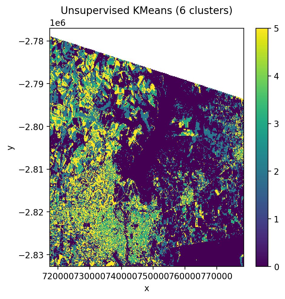
2. Unsupervised Classification (KMeans)#

No training labels needed. The algorithm identifies clusters directly from the pixel values.

[25]:

cl = Pipeline([('clf', KMeans(n_clusters=6, random_state=0))])

fig, ax = plt.subplots(dpi=200, figsize=(5, 5))

with gw.config.update(ref_res=150):
    with gw.open(l8_224078_20200518, nodata=0) as src:
        y = fit_predict(src, cl)
        y.plot(robust=True, ax=ax)

ax.set_title('Unsupervised KMeans (6 clusters)')
plt.tight_layout(pad=1)
plt.show()

3. Time Series Stacking with `stack_dim='band'`#

Stack multiple images along the band dimension. This concatenates spectral bands from each date into one long feature vector per pixel.

[26]:

fig, ax = plt.subplots(dpi=200, figsize=(5, 5))

with gw.config.update(ref_res=150):
    with gw.open(
        [l8_224078_20200518, l8_224078_20200518],
        stack_dim='band',
        nodata=0,
    ) as src:
        print('Band-stacked shape:', src.shape)
        print('Dims:', src.dims)
        y = fit_predict(src, pl, labels_poly, col='lc')
        print('\nPrediction shape:', y.shape)
        y.plot(robust=True, ax=ax)

ax.set_title('Band-stacked classification')
plt.tight_layout(pad=1)
plt.show()

Band-stacked shape: (6, 372, 408)
Dims: ('band', 'y', 'x')

Prediction shape: (1, 372, 408)

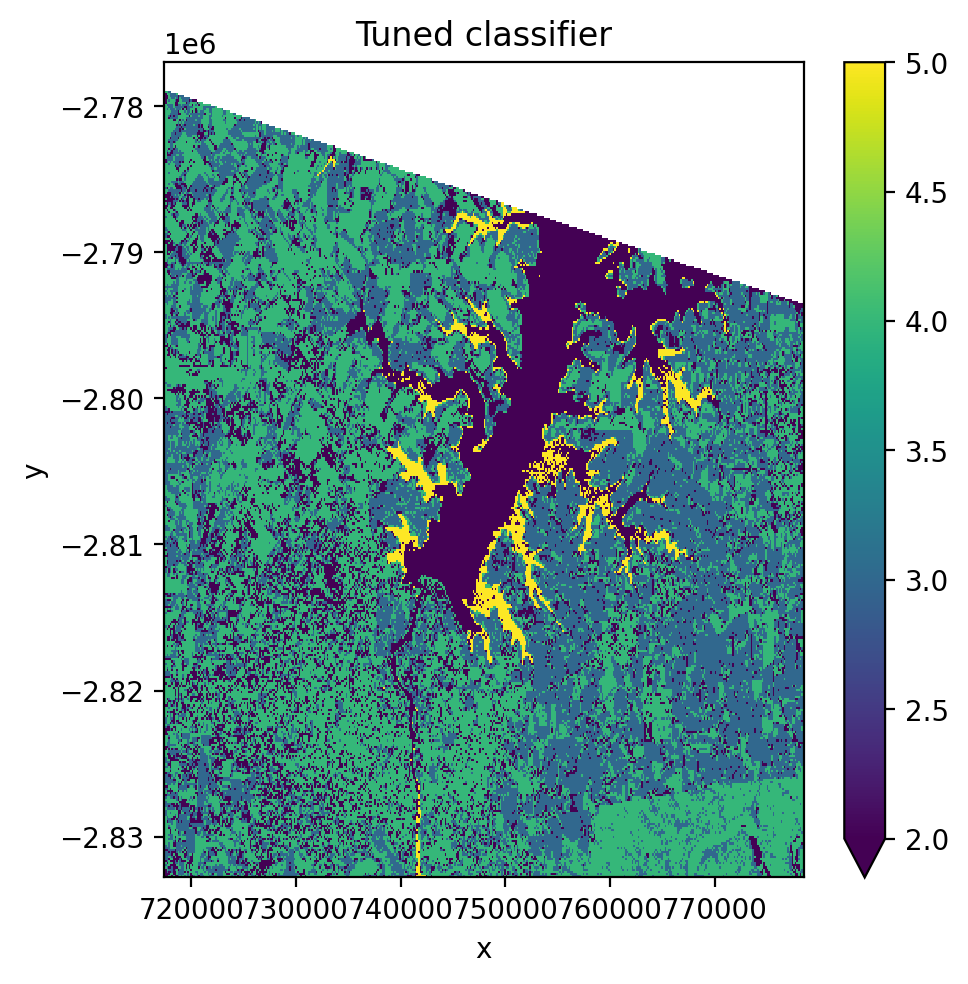
4. Cross-Validation & Hyperparameter Tuning#

Use GridSearchCV with CrossValidatorWrapper to tune pipeline hyperparameters.

[27]:

from sklearn.model_selection import GridSearchCV, KFold
from sklearn_xarray.model_selection import CrossValidatorWrapper

pl_cv = Pipeline(
    [
        ('scaler', StandardScaler()),
        ('pca', PCA()),
        ('clf', GaussianNB()),
    ]
)

cv = CrossValidatorWrapper(KFold())
gridsearch = GridSearchCV(
    pl_cv,
    cv=cv,
    scoring='balanced_accuracy',
    param_grid={
        'scaler__with_std': [True, False],
        'pca__n_components': [1, 2, 3],
    },
)

fig, ax = plt.subplots(dpi=200, figsize=(5, 5))

with gw.config.update(ref_res=150):
    with gw.open(l8_224078_20200518, nodata=0) as src:
        X, Xy, pipe = fit(src, pl_cv, labels_poly, col='lc')

        # Cross-validation and parameter tuning
        gridsearch.fit(*Xy)
        print('Best score:', gridsearch.best_score_)
        print('Best params:', gridsearch.best_params_)

        # Apply best parameters and predict
        pipe.set_params(**gridsearch.best_params_)
        y = predict(src, X, pipe)
        y.plot(robust=True, ax=ax)

ax.set_title('Tuned classifier')
plt.tight_layout(pad=1)
plt.show()

Best score: 0.3833404538104048
Best params: {'pca__n_components': 3, 'scaler__with_std': True}

5. Time-Dimensioned Data with `temporal_mode`#

When you open multiple images with stack_dim='time', the data has shape (time, band, y, x). This is the format returned by STAC queries and multi-date gw.open() calls.

The temporal_mode parameter controls how time is handled during classification:

`temporal_mode`	Samples	Features	Output shape
`'panel'` (default)	T × H × W	B	`(time, band='targ', y, x)` — one prediction per pixel per time step
`'flatten'`	H × W	T × B	`(band='targ', y, x)` — one prediction per pixel using all time steps as features

Inspect time-stacked data#

[28]:

with gw.config.update(ref_res=150):
    with gw.open(
        [l8_224078_20200518, l8_224078_20200518],
        stack_dim='time',
    ) as src:
        print('Time-stacked data:')
        print(f'  Shape: {src.shape}')
        print(f'  Dims:  {src.dims}')
        print(f'  Time coords: {src.time.values}')
        print(f'  Band coords: {src.band.values}')

Time-stacked data:
  Shape: (2, 3, 372, 408)
  Dims:  ('time', 'band', 'y', 'x')
  Time coords: [1 2]
  Band coords: [1 2 3]

Panel mode (`temporal_mode='panel'`)#

Each pixel-time combination is treated as an independent sample with B spectral features. The output retains the time dimension, giving one prediction map per time step.

[29]:

pl_panel = Pipeline(
    [
        ('scaler', StandardScaler()),
        ('pca', PCA()),
        ('clf', GaussianNB()),
    ]
)

with gw.config.update(ref_res=150):
    with gw.open(
        [l8_224078_20200518, l8_224078_20200518],
        stack_dim="time",
        nodata=0,
    ) as src:
        y_panel = fit_predict(
            src,
            pl_panel,
            labels_point,
            col='lc',
            temporal_mode='panel',
        )

print('Panel output:')
print(f'  Shape: {y_panel.shape}')
print(f'  Dims:  {y_panel.dims}')
print(f'  Time dim preserved: {"time" in y_panel.dims}')

# Plot each time step
fig, axes = plt.subplots(1, 2, dpi=200, figsize=(10, 5))
for i, ax in enumerate(axes):
    y_panel.isel(time=i).plot(robust=True, ax=ax)
    ax.set_title(f'Panel prediction \u2013 time step {i}')
plt.tight_layout(pad=1)
plt.show()

# Since both time steps use the same image, predictions should match
print(
    '\nTime steps identical:',
    np.allclose(
        y_panel.isel(time=0).values,
        y_panel.isel(time=1).values,
        equal_nan=True,
    ),
)

Panel output:
  Shape: (2, 1, 372, 408)
  Dims:  ('time', 'band', 'y', 'x')
  Time dim preserved: True


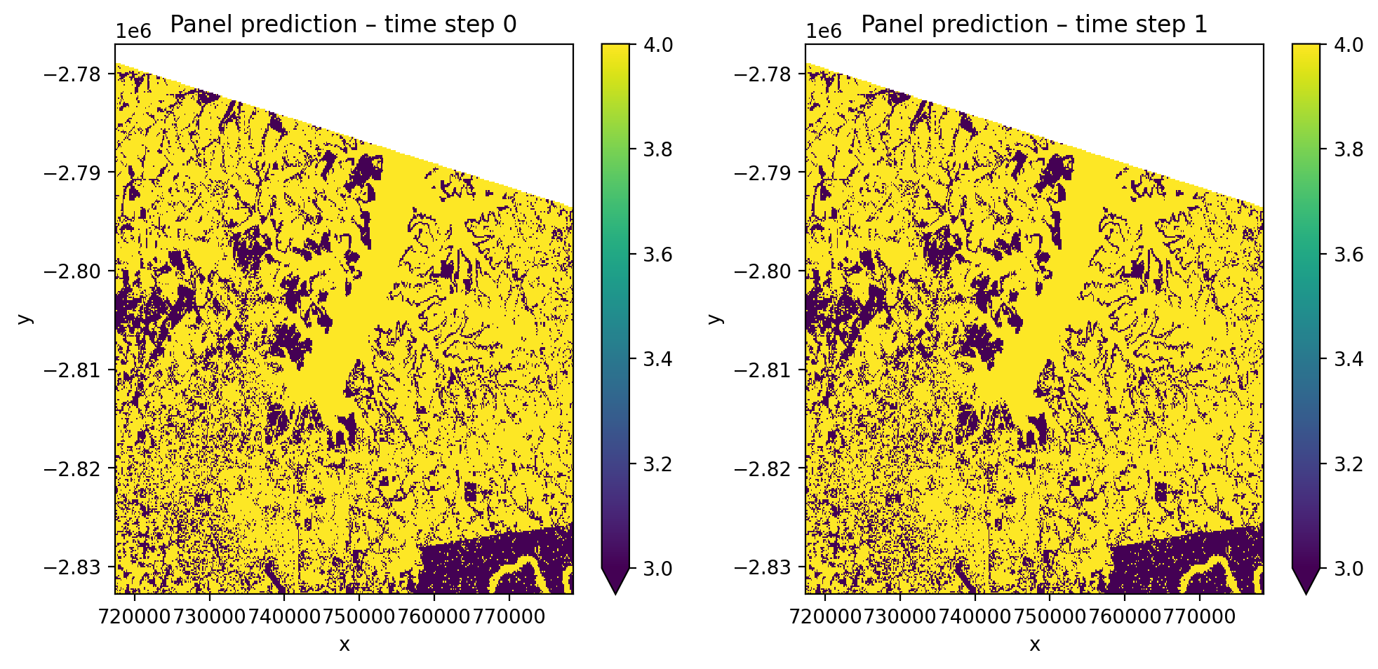
Time steps identical: True

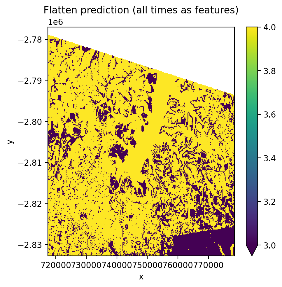
Flatten mode (`temporal_mode='flatten'`)#

All time steps are flattened into the band dimension, creating T×B features per pixel. This produces a single prediction map regardless of how many time steps exist.

[30]:

# Use PCA with n_components=1 since we have more features (T*B) than samples
pl_flatten = Pipeline(
    [
        ('scaler', StandardScaler()),
        ('pca', PCA(n_components=1)),
        ('clf', GaussianNB()),
    ]
)

with gw.config.update(ref_res=150):
    with gw.open(
        [l8_224078_20200518, l8_224078_20200518],
        stack_dim="time",
        nodata=0,
    ) as src:
        y_flat = fit_predict(
            src,
            pl_flatten,
            labels_point,
            col='lc',
            temporal_mode='flatten',
        )

print('Flatten output:')
print(f'  Shape: {y_flat.shape}')
print(f'  Dims:  {y_flat.dims}')
print(f'  Time dim removed: {"time" not in y_flat.dims}')

fig, ax = plt.subplots(dpi=200, figsize=(5, 5))
y_flat.plot(robust=True, ax=ax)
ax.set_title('Flatten prediction (all times as features)')
plt.tight_layout(pad=1)
plt.show()

Flatten output:
  Shape: (1, 372, 408)
  Dims:  ('band', 'y', 'x')
  Time dim removed: True

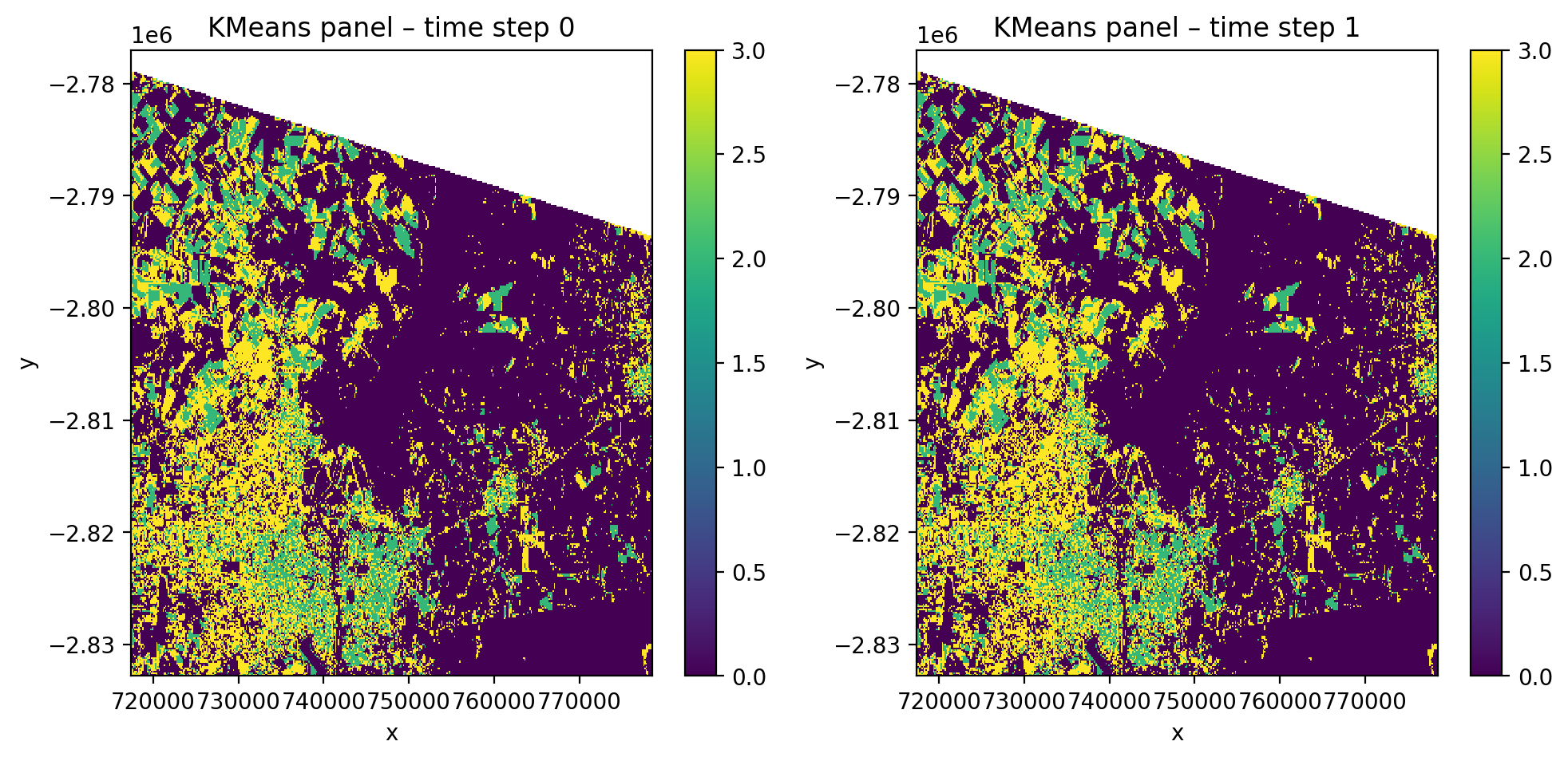
Unsupervised clustering with time-stacked data#

[31]:

cl_time = Pipeline(
    [
        ('scaler', StandardScaler()),
        ('clf', KMeans(n_clusters=4, random_state=0)),
    ]
)

with gw.config.update(ref_res=150):
    with gw.open(
        [l8_224078_20200518, l8_224078_20200518],
        stack_dim='time',
        nodata=0,
    ) as src:
        y_cl = fit_predict(
            data=src,
            clf=cl_time,
            temporal_mode='panel',
        )

print('Unsupervised panel output:')
print(f'  Shape: {y_cl.shape}')
print(f'  Dims:  {y_cl.dims}')

fig, axes = plt.subplots(1, 2, dpi=200, figsize=(10, 5))
for i, ax in enumerate(axes):
    y_cl.isel(time=i).plot(robust=True, ax=ax)
    ax.set_title(f'KMeans panel \u2013 time step {i}')
plt.tight_layout(pad=1)
plt.show()

Unsupervised panel output:
  Shape: (2, 1, 372, 408)
  Dims:  ('time', 'band', 'y', 'x')

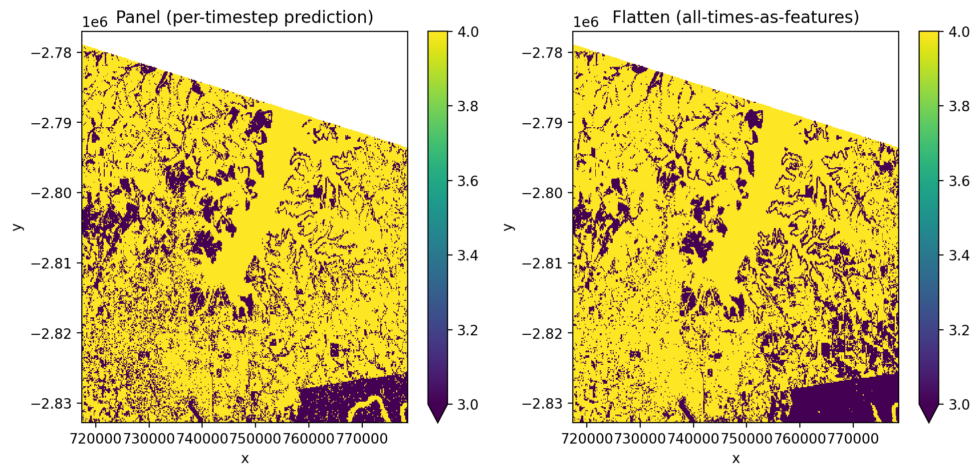
Compare panel vs flatten side by side#

[32]:

fig, axes = plt.subplots(1, 2, dpi=200, figsize=(10, 5))

y_panel.isel(time=0).plot(robust=True, ax=axes[0])
axes[0].set_title('Panel (per-timestep prediction)')

y_flat.plot(robust=True, ax=axes[1])
axes[1].set_title('Flatten (all-times-as-features)')

plt.tight_layout(pad=1)
plt.show()

Notes#

``n_classes`` is auto-inferred from the label column during fit(). You never need to specify it.
Nodata handling: Pixels with nodata values are automatically masked as NaN in predictions.
``ref_res`` controls the output resolution. Use coarser resolution (e.g., 150–300m) for faster demos.
For production workflows, use more training data and full-resolution imagery.
Save predictions with y.gw.save('classification.tif', overwrite=True)
See the dl_classifiers.ipynb notebook for deep learning classifiers (TabNet, L-TAE, TorchGeo).
See the stac.ipynb notebook for downloading satellite imagery from cloud catalogs.

Machine Learning Classification in GeoWombat

Contents