Machine learning#

GeoWombat’s ML module works with any scikit-learn compatible classifier or pipeline. Pass a classifier to fit(), predict(), or fit_predict() and it will be applied to the raster data as an xarray DataArray.

To install ML dependencies:

pip install "geowombat[ml]"

Recommended classifiers for remote sensing#

Supervised#

Classifier	Module	Notes
Random Forest	`sklearn.ensemble.RandomForestClassifier`	Most widely used in remote sensing; handles high-dimensional data well, robust to noise
LightGBM	`lightgbm.LGBMClassifier`	Fast gradient boosting; strong accuracy with large datasets, supports categorical features
Gradient Boosted Trees	`sklearn.ensemble.GradientBoostingClassifier`	Strong accuracy; slower than LightGBM on large datasets
Support Vector Machine	`sklearn.svm.SVC`	Effective in high-dimensional spaces; works well with small training sets
Gaussian Naive Bayes	`sklearn.naive_bayes.GaussianNB`	Fast and simple baseline; assumes feature independence
k-Nearest Neighbors	`sklearn.neighbors.KNeighborsClassifier`	Non-parametric; useful for complex class boundaries

Unsupervised#

Classifier	Module	Notes
K-Means	`sklearn.cluster.KMeans`	Standard clustering; fast, works well for spectrally distinct classes
Mini-Batch K-Means	`sklearn.cluster.MiniBatchKMeans`	Faster K-Means variant for large rasters
Gaussian Mixture Model	`sklearn.mixture.GaussianMixture`	Soft clustering; models class overlap better than K-Means

Setup#

import geowombat as gw
from geowombat.data import (
    l8_224078_20200518,
    l8_224078_20200518_points,
    stac_training,
)
from geowombat.ml import fit, predict, fit_predict

import geopandas as gpd
import matplotlib.pyplot as plt
import numpy as np
from sklearn.pipeline import Pipeline
from sklearn.preprocessing import LabelEncoder, StandardScaler
from sklearn.decomposition import PCA
from sklearn.naive_bayes import GaussianNB
from sklearn.cluster import KMeans

# Polygon labels (integer 'lc' column, EPSG:4326)
labels_poly = gpd.read_file(stac_training)

# Point labels (need LabelEncoder for string names)
le = LabelEncoder()
labels_point = gpd.read_file(l8_224078_20200518_points)
labels_point['lc'] = le.fit(labels_point.name).transform(labels_point.name)
labels_point = labels_point.drop(columns=['name'])

Nodata handling#

By default, fit_predict() and predict() mask nodata pixels in the output with NaN (mask_nodataval=True). This prevents nodata regions from being assigned a class label.

When opening a file with gw.open(..., nodata=0), GeoWombat builds a binary nodata mask from the original file before warping. This mask is attached as the _nodata_mask coordinate and survives reprojection and time-stacking. The _mask_nodata() method uses it to replace predictions at nodata locations with NaN.

with gw.config.update(ref_res=150):
    with gw.open(l8_224078_20200518, nodata=0) as src:
        # _nodata_mask is automatically attached
        print('Has nodata mask:', '_nodata_mask' in src.coords)

        # mask_nodataval=True (default) masks nodata in predictions
        y = fit_predict(src, pl, labels_poly, col='lc')

To disable nodata masking, pass mask_nodataval=False. This is useful when you want to handle masking yourself or inspect raw predictions.

Supervised classification#

Using `fit()` then `predict()` (two-step)#

pl = Pipeline([
    ('scaler', StandardScaler()),
    ('pca', PCA()),
    ('clf', GaussianNB()),
])

with gw.config.update(ref_res=150):
    with gw.open(l8_224078_20200518, nodata=0) as src:
        X, Xy, clf = fit(src, pl, labels_poly, col='lc')
        y = predict(src, X, clf)
        y.plot(robust=True)

Supervised classification (fit + predict)

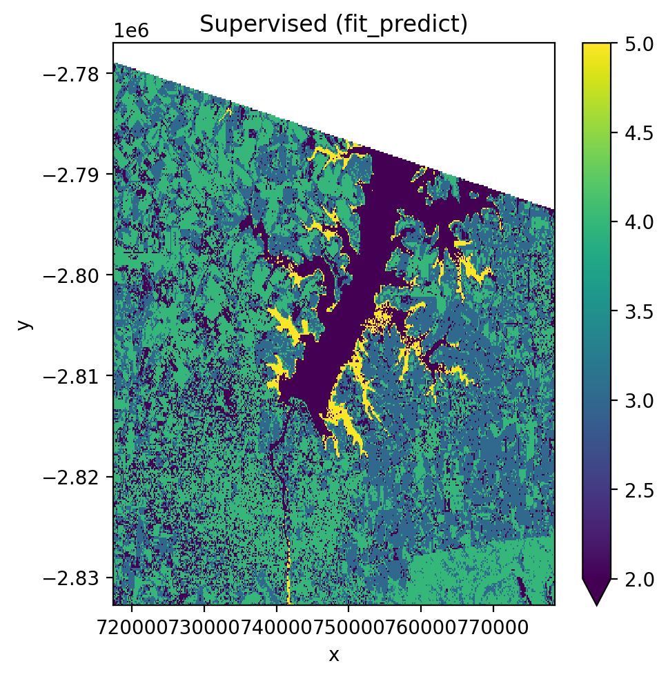
Using `fit_predict()` (one-step)#

with gw.config.update(ref_res=150):
    with gw.open(l8_224078_20200518, nodata=0) as src:
        y = fit_predict(src, pl, labels_poly, col='lc')
        y.plot(robust=True)

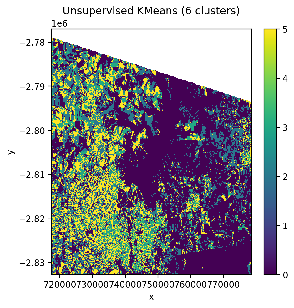
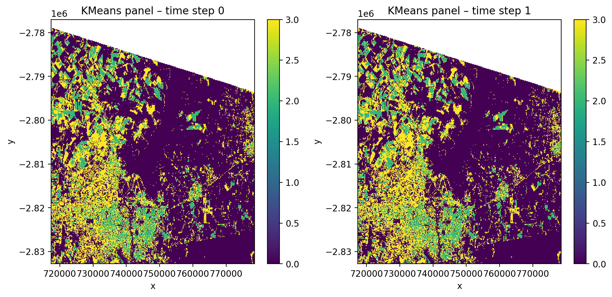
Unsupervised classification (KMeans)#

No training labels needed. The algorithm identifies clusters directly from the pixel values.

cl = Pipeline([('clf', KMeans(n_clusters=6, random_state=0))])

with gw.config.update(ref_res=150):
    with gw.open(l8_224078_20200518, nodata=0) as src:
        y = fit_predict(src, cl)
        y.plot(robust=True)

Band-stacked classification#

Stack multiple images along the band dimension with stack_dim='band'. This concatenates spectral bands from each date into one long feature vector per pixel.

with gw.config.update(ref_res=150):
    with gw.open(
        [l8_224078_20200518, l8_224078_20200518],
        stack_dim='band',
        nodata=0,
    ) as src:
        print('Band-stacked shape:', src.shape)
        y = fit_predict(src, pl, labels_poly, col='lc')
        y.plot(robust=True)

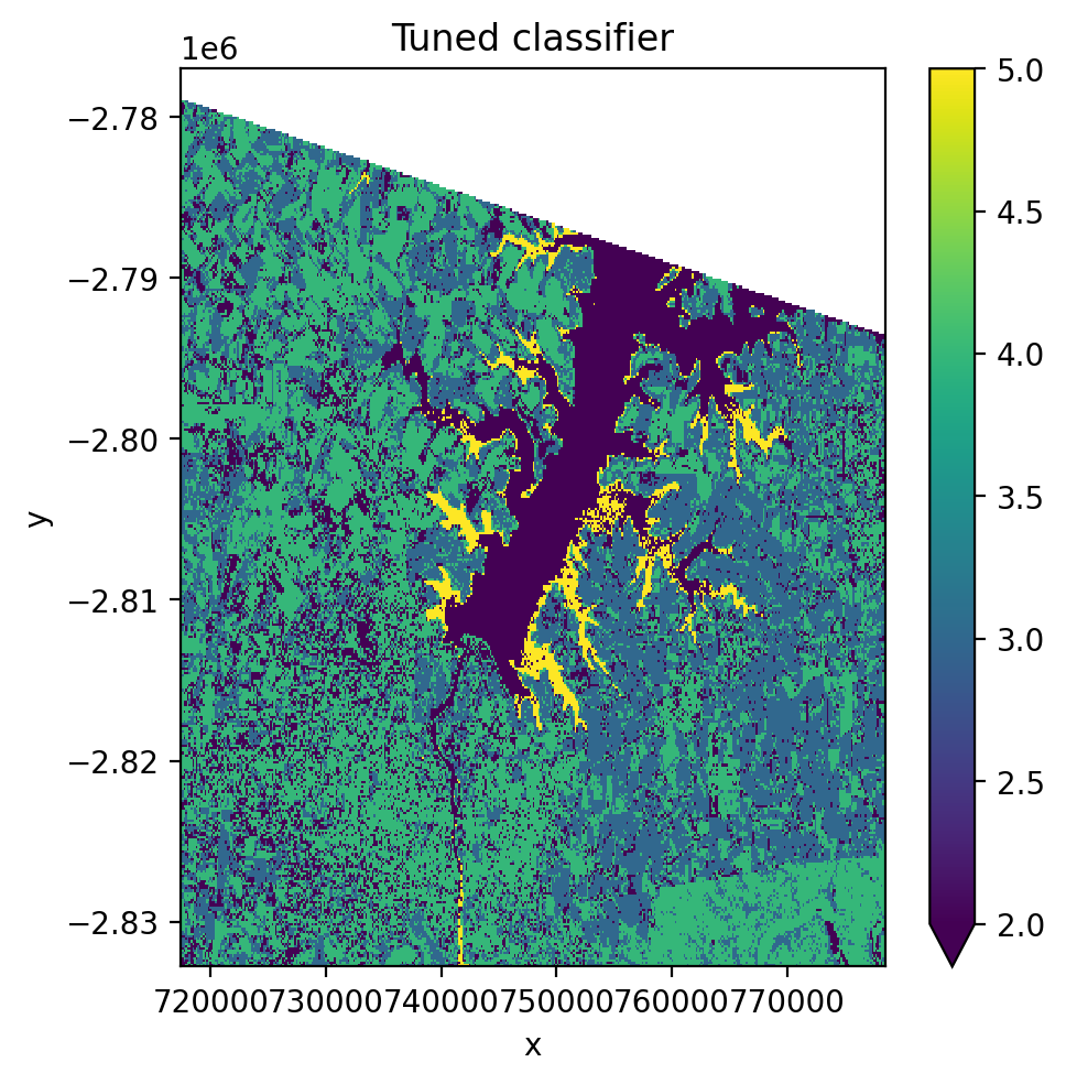
Cross-validation and hyperparameter tuning#

Use GridSearchCV with CrossValidatorWrapper to tune pipeline hyperparameters.

from sklearn.model_selection import GridSearchCV, KFold
from sklearn_xarray.model_selection import CrossValidatorWrapper

cv = CrossValidatorWrapper(KFold())
gridsearch = GridSearchCV(
    pl,
    cv=cv,
    scoring='balanced_accuracy',
    param_grid={
        'scaler__with_std': [True, False],
        'pca__n_components': [1, 2, 3],
    },
)

with gw.config.update(ref_res=150):
    with gw.open(l8_224078_20200518, nodata=0) as src:
        X, Xy, pipe = fit(src, pl, labels_poly, col='lc')

        gridsearch.fit(*Xy)
        print('Best params:', gridsearch.best_params_)

        pipe.set_params(**gridsearch.best_params_)
        y = predict(src, X, pipe)
        y.plot(robust=True)

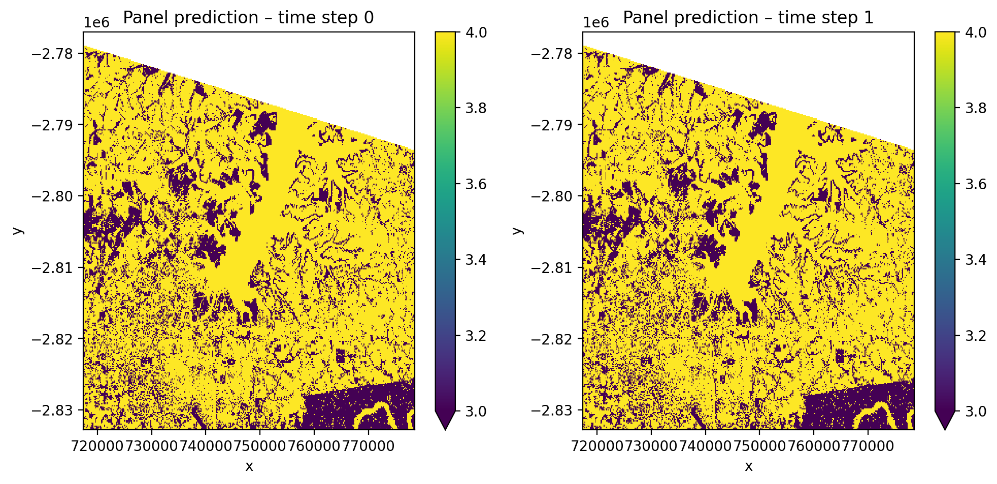
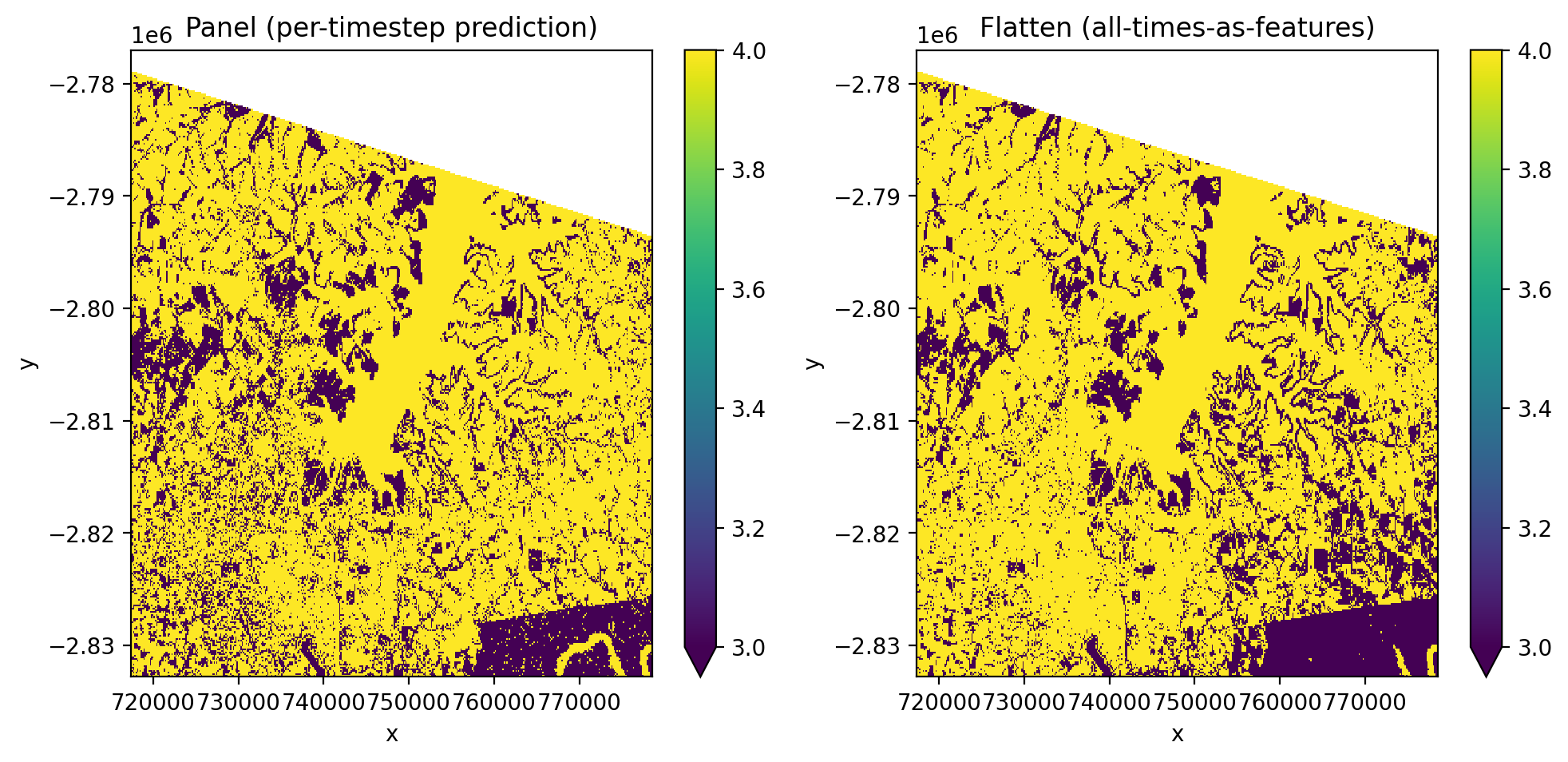
Time-stacked classification with `temporal_mode`#

When opening multiple images with stack_dim='time', the data has shape (time, band, y, x). This is the format returned by STAC queries and multi-date gw.open() calls. The temporal_mode parameter controls how time is handled during classification:

'panel' (default) — each pixel-time is an independent sample with B spectral features. Output retains the time dimension with one prediction per time step.
'flatten' — all time steps are flattened into the band dimension, creating T×B features per pixel. Output has no time dimension.

Input	`temporal_mode`	Features	Output shape
`(time=T, band=B, y, x)`	`'panel'`	B	`(time=T, band='targ', y, x)`
`(time=T, band=B, y, x)`	`'flatten'`	T × B	`(band='targ', y, x)`

Panel mode#

Each pixel-time combination is treated as an independent sample. The output retains the time dimension, giving one prediction map per time step. Nodata pixels are masked automatically (mask_nodataval=True by default).

pl_panel = Pipeline([
    ('scaler', StandardScaler()),
    ('pca', PCA()),
    ('clf', GaussianNB()),
])

with gw.config.update(ref_res=150):
    with gw.open(
        [l8_224078_20200518, l8_224078_20200518],
        stack_dim='time',
        nodata=0,
    ) as src:
        y_panel = fit_predict(
            src, pl_panel, labels_point, col='lc',
            temporal_mode='panel',
        )

print(f'Shape: {y_panel.shape}')  # (2, 1, 372, 408)
print(f'Dims:  {y_panel.dims}')   # ('time', 'band', 'y', 'x')

# Since both time steps use the same image, predictions should match
print('Time steps identical:',
      np.allclose(y_panel.isel(time=0).values,
                  y_panel.isel(time=1).values, equal_nan=True))

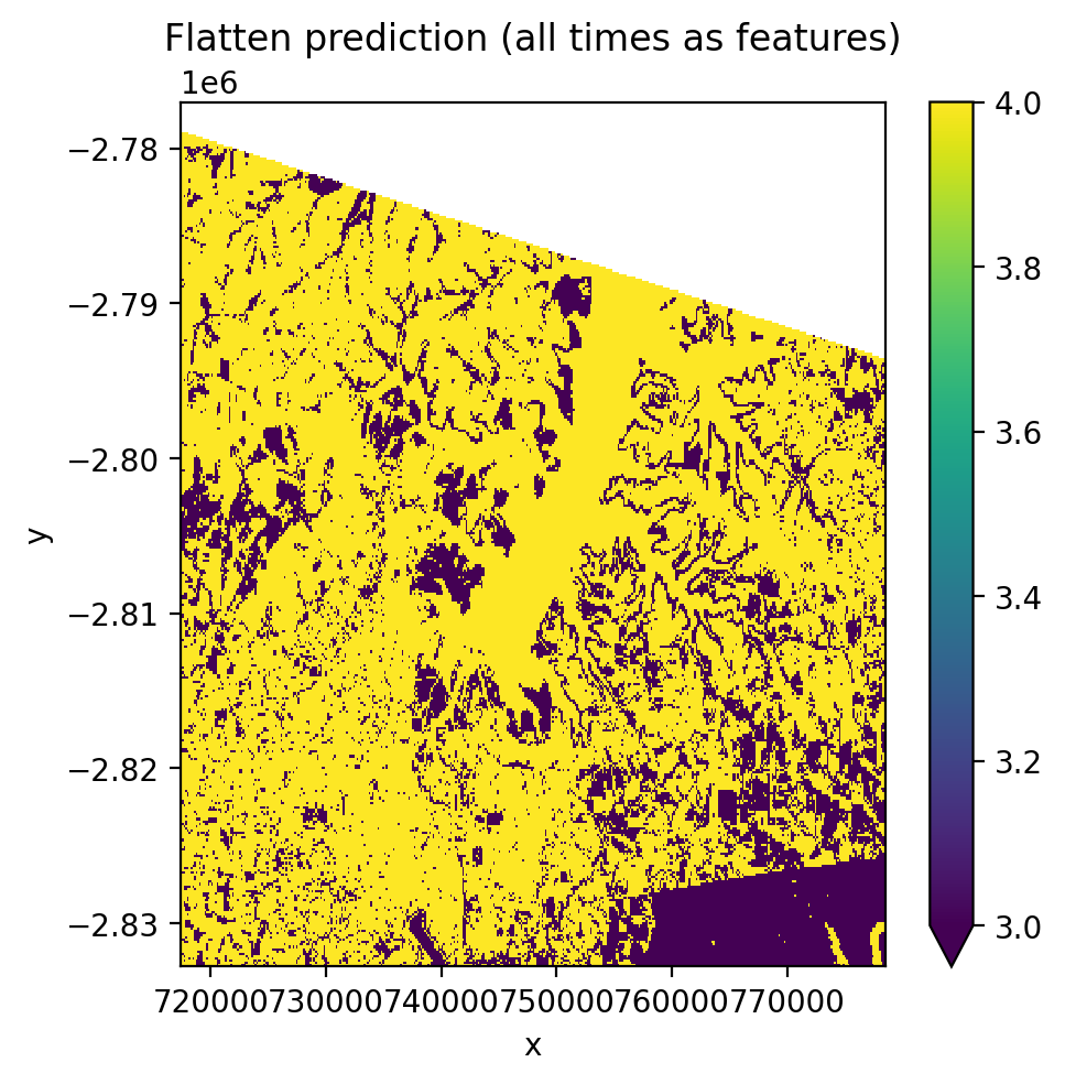
Flatten mode#

All time steps are flattened into the band dimension, creating T×B features per pixel. This produces a single prediction map regardless of how many time steps exist.

pl_flatten = Pipeline([
    ('scaler', StandardScaler()),
    ('pca', PCA(n_components=1)),
    ('clf', GaussianNB()),
])

with gw.config.update(ref_res=150):
    with gw.open(
        [l8_224078_20200518, l8_224078_20200518],
        stack_dim='time',
        nodata=0,
    ) as src:
        y_flat = fit_predict(
            src, pl_flatten, labels_point, col='lc',
            temporal_mode='flatten',
        )

print(f'Shape: {y_flat.shape}')  # (1, 372, 408)
print(f'Dims:  {y_flat.dims}')   # ('band', 'y', 'x')

Flatten mode prediction (all times as features)

Unsupervised clustering with time-stacked data#

cl_time = Pipeline([
    ('scaler', StandardScaler()),
    ('clf', KMeans(n_clusters=4, random_state=0)),
])

with gw.config.update(ref_res=150):
    with gw.open(
        [l8_224078_20200518, l8_224078_20200518],
        stack_dim='time',
        nodata=0,
    ) as src:
        y_cl = fit_predict(
            data=src, clf=cl_time,
            temporal_mode='panel',
        )

Compare panel vs flatten#

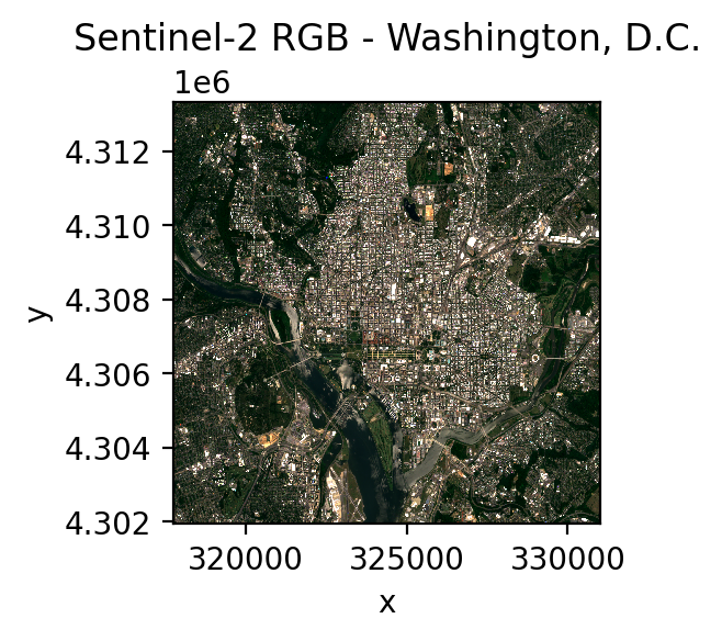
Classification with STAC satellite imagery#

GeoWombat can stream satellite imagery directly from cloud catalogs using open_stac(). The returned data has shape (time, band, y, x) and works directly with fit_predict(). No file downloads are needed — data is read from Cloud Optimized GeoTIFFs (COGs) on the fly.

To install STAC dependencies:

pip install "geowombat[stac]"

Search and load imagery#

Use open_stac() to search a STAC catalog and load the matching scenes. Set compute=True to download the data into memory with a progress bar.

from geowombat.core.stac import open_stac

# Search for Sentinel-2 imagery over Washington, DC
data, df = open_stac(
    stac_catalog="element84_v1",
    collection="sentinel_s2_l2a",
    bounds=(-77.1, 38.85, -76.95, 38.95),
    epsg=32618,
    bands=["blue", "green", "red", "nir"],
    start_date="2023-06-01",
    end_date="2023-07-31",
    cloud_cover_perc=20,
    resolution=100.0,
    chunksize=256,
    max_items=2,
    compute=True,
)

print(f"Shape: {data.shape}")   # (2, 4, 115, 134)
print(f"Dims:  {data.dims}")    # ('time', 'band', 'y', 'x')

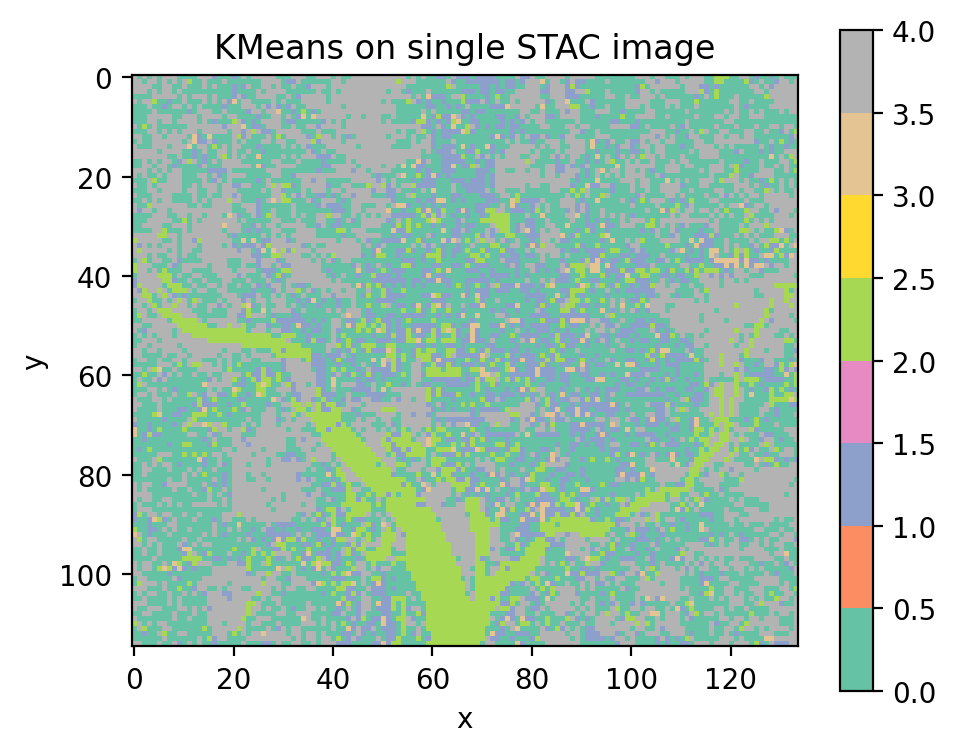
Unsupervised classification on a single STAC image#

Select one time step with .isel(time=0) and pass it directly to fit_predict(). No training labels are needed for unsupervised classifiers.

from sklearn.cluster import MiniBatchKMeans

cl_stac = Pipeline([
    ("clf", MiniBatchKMeans(n_clusters=5, random_state=0)),
])

single_image = data.isel(time=0)
y_single = fit_predict(data=single_image, clf=cl_stac)
y_single.plot(robust=True)

Save prediction output#

y.gw.save('output.tif', overwrite=True)

Machine learning

Contents