Accessing Satellite Imagery with STAC#

STAC (SpatioTemporal Asset Catalog) is an open standard for cataloging satellite imagery in the cloud. GeoWombat can search STAC catalogs, download imagery on-the-fly, apply cloud masking, and create temporal composites — all with a few function calls.

This notebook covers:

Searching & downloading imagery with open_stac()
Supported catalogs and collections
Automatic cloud masking with mask_data=True
Harmonized Landsat Sentinel-2 (HLS) data
Cloud-free composites with composite_stac()
Classification on STAC data

Requirements: pip install "geowombat[stac]"

Setup#

[ ]:

import os
os.environ['CPL_LOG'] = '/dev/null'  # suppress GDAL warnings

import warnings
import matplotlib.pyplot as plt
import numpy as np

warnings.filterwarnings('ignore', category=(DeprecationWarning))
warnings.filterwarnings('ignore', category=(FutureWarning))
warnings.filterwarnings('ignore', category=(UserWarning))

1. Searching & Downloading with `open_stac()`#

open_stac() searches a STAC catalog for imagery matching your criteria and returns an xarray DataArray with shape (time, band, y, x).

Key parameters:

Parameter	Description
`stac_catalog`	Catalog to search (see table below)
`collection`	Data collection name
`bounds`	Bounding box as `(west, south, east, north)` in EPSG:4326
`epsg`	Output CRS EPSG code
`bands`	List of band names (e.g., `['red', 'green', 'blue', 'nir']`)
`start_date` / `end_date`	Date range for search
`cloud_cover_perc`	Maximum cloud cover percentage
`resolution`	Output pixel size in CRS units (meters)
`max_items`	Maximum number of scenes to return
`chunksize`	Dask chunk size (default 256)
`compute`	If `True`, load into memory immediately

[2]:

from geowombat.core.stac import open_stac

# Search for Sentinel-2 imagery over Washington, DC
data, df = open_stac(
    stac_catalog='element84_v1',
    collection='sentinel_s2_l2a',
    bounds=(-77.1, 38.85, -76.95, 38.95),  # (west, south, east, north)
    epsg=32618,
    bands=['blue', 'green', 'red', 'nir'],
    start_date='2023-06-01',
    end_date='2023-07-31',
    cloud_cover_perc=20,
    resolution=100.0,
    chunksize=256,
    max_items=2,
)

print(f'Shape: {data.shape}')
print(f'Dims:  {data.dims}')
print(f'Times: {data.time.values}')
print(f'Bands: {data.band.values}')
print(f'Type:  {type(data)}')

/home/mmann1123/miniconda3/envs/geowombat_dev/lib/python3.11/site-packages/tqdm/auto.py:21: TqdmWarning: IProgress not found. Please update jupyter and ipywidgets. See https://ipywidgets.readthedocs.io/en/stable/user_install.html
  from .autonotebook import tqdm as notebook_tqdm

Searching element84_v1 for sentinel_s2_l2a...
Found 1 items.

Downloading sentinel_s2_l2a: 100%|██████████| 9/9 [00:01<00:00,  4.74it/s]

Shape: (1, 4, 115, 134)
Dims:  ('time', 'band', 'y', 'x')
Times: ['2023-06-02T16:12:23.667000000']
Bands: ['blue' 'green' 'red' 'nir']
Type:  <class 'xarray.core.dataarray.DataArray'>

[3]:

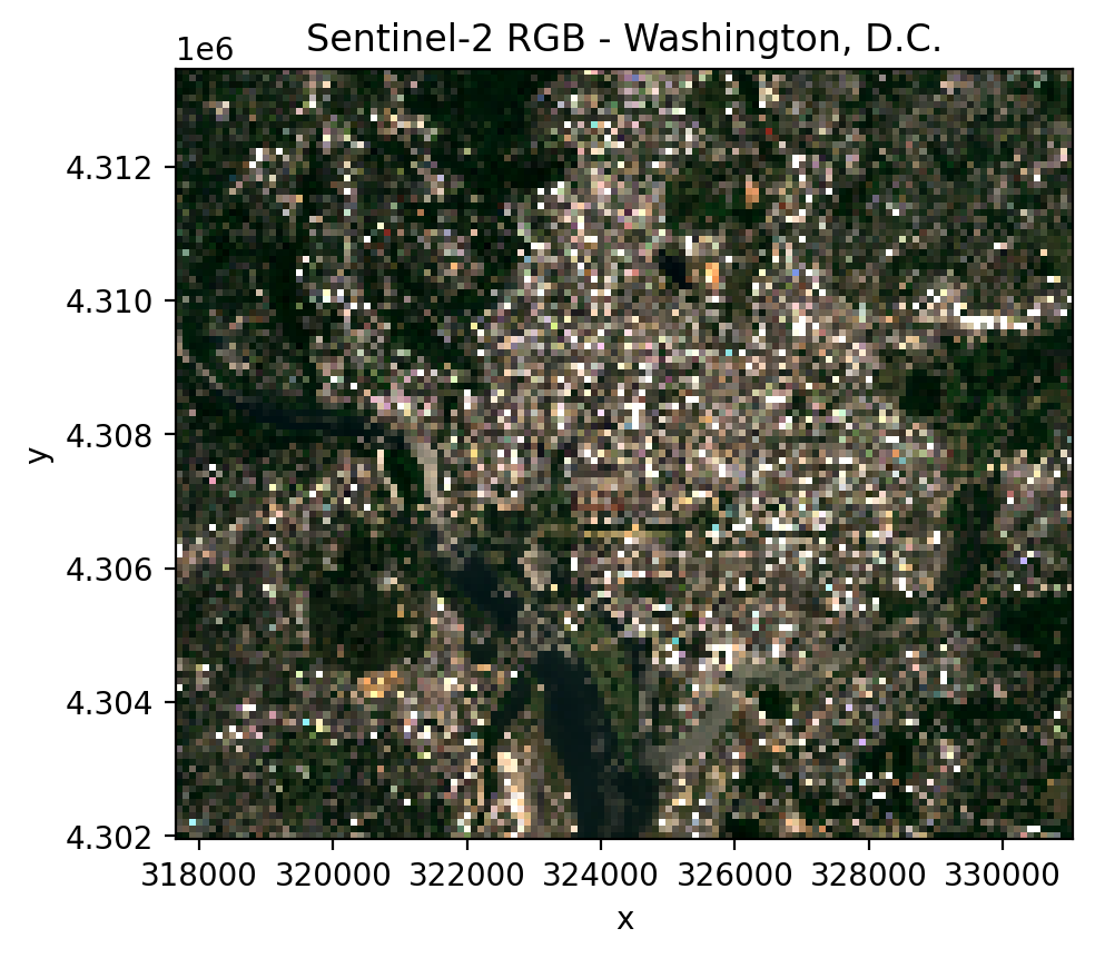
fig, ax = plt.subplots(dpi=200, figsize=(5, 5))
data.sel(time=data.time[0], band=['red', 'green', 'blue']).plot.imshow(
    robust=True, ax=ax
)
ax.set_title('Sentinel-2 RGB - Washington, D.C.')
ax.set_aspect('equal')
plt.tight_layout(pad=1)
plt.show()

2. Supported Catalogs & Collections#

GeoWombat supports four STAC catalogs:

Catalog	`stac_catalog`	Collections	Auth
Element 84	`element84_v1`	`sentinel_s2_l2a`, `sentinel_s2_l1c`, `sentinel_s1_l1c`, `landsat_c2_l2`, `cop_dem_glo_30`, `naip`	None
Microsoft Planetary Computer	`microsoft_v1`	`landsat_c2_l2`, `landsat_c2_l1`, `sentinel_s2_l2a`, `sentinel_s1_l1c`, `usda_cdl`, `io_lulc`, `esa_worldcover`, `cop_dem_glo_30`	None
NASA LP DAAC	`nasa_lp_cloud`	`hls_l30`, `hls_s30`	`~/.netrc`

Use collection='hls' with composite_stac() to query both HLS L30 and S30 simultaneously.

Band naming#

Use friendly band names: red, green, blue, nir, swir1, swir2, etc. GeoWombat maps these to the correct asset names for each collection.

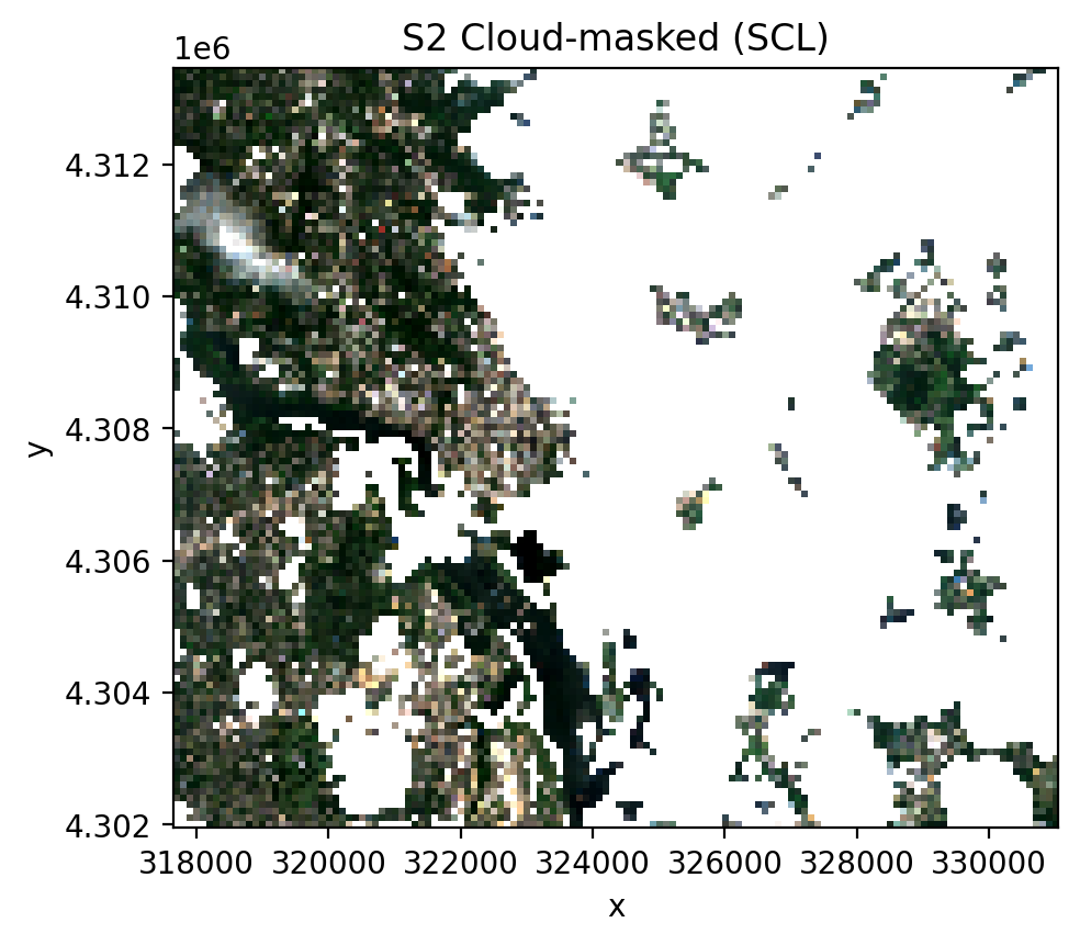
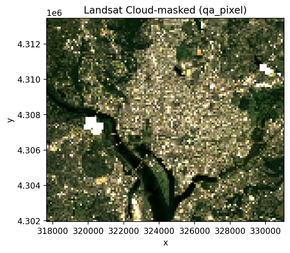
3. Cloud Masking with `mask_data=True`#

When mask_data=True, open_stac() automatically loads the appropriate QA band and masks bad pixels:

Sentinel-2: Loads the SCL (Scene Classification Layer) band and masks clouds, cloud shadows, cirrus, saturated pixels, and nodata
Landsat: Loads the qa_pixel band and applies bitmask for clouds, cloud shadows, cirrus, snow, and fill

You do not need to include scl or qa_pixel in your bands list — they are auto-injected.

Sentinel-2 cloud masking#

[4]:

# Sentinel-2 with cloud masking via SCL band
data_s2_masked, df_s2 = open_stac(
    stac_catalog='element84_v1',
    collection='sentinel_s2_l2a',
    bounds=(-77.1, 38.85, -76.95, 38.95),
    epsg=32618,
    bands=['blue', 'green', 'red', 'nir'],
    start_date='2023-06-01',
    end_date='2023-07-31',
    cloud_cover_perc=50,
    resolution=100.0,
    chunksize=256,
    max_items=2,
    mask_data=True,   # <-- auto-loads SCL, masks clouds
    compute=True,
)

print(f'Masked shape: {data_s2_masked.shape}')
print(f'Bands: {list(data_s2_masked.band.values)}')
print(f'NaN fraction (masked): {float(np.isnan(data_s2_masked.values).mean()):.3f}')

fig, ax = plt.subplots(dpi=200, figsize=(5, 5))
t0 = data_s2_masked.time[0]
data_s2_masked.sel(time=t0, band=['red', 'green', 'blue']).plot.imshow(
    robust=True, ax=ax
)
ax.set_title('S2 Cloud-masked (SCL)')
ax.set_aspect('equal')
plt.tight_layout(pad=1)
plt.show()

Searching element84_v1 for sentinel_s2_l2a...
Found 2 items.

Downloading sentinel_s2_l2a: 100%|██████████| 41/41 [00:03<00:00, 11.83it/s]

Masked shape: (2, 4, 115, 134)
Bands: ['blue', 'green', 'red', 'nir']
NaN fraction (masked): 0.290

Landsat cloud masking#

[5]:

# Landsat with cloud masking via qa_pixel band
data_ls_masked, df_ls = open_stac(
    stac_catalog='microsoft_v1',
    collection='landsat_c2_l2',
    bounds=(-77.1, 38.85, -76.95, 38.95),
    epsg=32618,
    bands=['red', 'green', 'blue'],
    start_date='2023-06-01',
    end_date='2023-07-31',
    cloud_cover_perc=50,
    resolution=100.0,
    chunksize=256,
    max_items=2,
    mask_data=True,   # <-- auto-loads qa_pixel, masks clouds
    compute=True,
)

print(f'Landsat masked shape: {data_ls_masked.shape}')
print(f'Bands: {list(data_ls_masked.band.values)}')
print(f'NaN fraction (masked): {float(np.isnan(data_ls_masked.values).mean()):.3f}')

fig, ax = plt.subplots(dpi=200, figsize=(5, 5))
data_ls_masked.sel(time=data_ls_masked.time[0]).plot.imshow(
    robust=True, ax=ax
)
ax.set_title('Landsat Cloud-masked (qa_pixel)')
ax.set_aspect('equal')
plt.tight_layout(pad=1)
plt.show()

Searching microsoft_v1 for landsat_c2_l2...
Found 2 items.

Downloading landsat_c2_l2: 100%|██████████| 29/29 [00:02<00:00, 11.29it/s]

Landsat masked shape: (2, 3, 115, 134)
Bands: ['red', 'green', 'blue']
NaN fraction (masked): 0.006

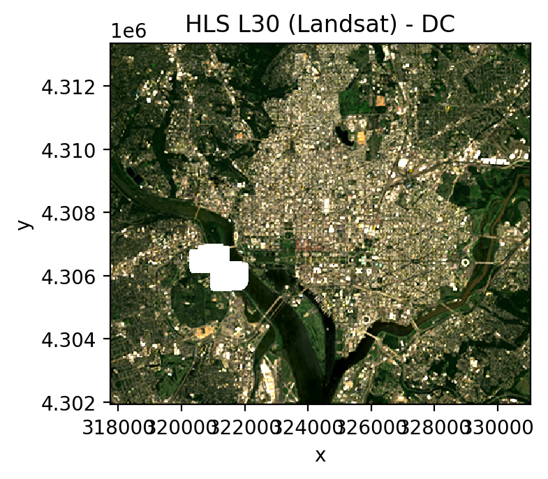
4. Harmonized Landsat Sentinel-2 (HLS)#

NASA’s HLS provides BRDF-normalized, harmonized 30m surface reflectance from both Landsat and Sentinel-2 on a common grid. Available via the NASA CMR STAC:

``hls_l30``: Landsat OLI 30m (HLSL30 v2.0)
``hls_s30``: Sentinel-2 MSI 30m (HLSS30 v2.0)

Credentials required: Create a ~/.netrc file with NASA Earthdata login:

machine urs.earthdata.nasa.gov login <your_username> password <your_password>

[6]:

# HLS L30 (Landsat-derived, 30m)
try:
    data_hls_l30, df_hls_l30 = open_stac(
        stac_catalog='nasa_lp_cloud',
        collection='hls_l30',
        bounds=(-77.1, 38.85, -76.95, 38.95),
        epsg=32618,
        bands=['red', 'green', 'blue', 'nir'],
        start_date='2023-06-01',
        end_date='2023-07-31',
        cloud_cover_perc=30,
        resolution=30.0,
        max_items=3,
        mask_data=True,
    )

    print(f'HLS L30 shape: {data_hls_l30.shape}')
    print(f'Bands: {list(data_hls_l30.band.values)}')
    print(f'Times: {data_hls_l30.time.values}')

    fig, ax = plt.subplots(dpi=200, figsize=(4, 4))
    data_hls_l30.sel(
        time=data_hls_l30.time[0], band=['red', 'green', 'blue']
    ).plot.imshow(robust=True, ax=ax)
    ax.set_title('HLS L30 (Landsat) - DC')
    ax.set_aspect('equal')
    plt.tight_layout(pad=1)
    plt.show()
except Exception as e:
    print(f'HLS L30 failed (need ~/.netrc credentials): {e}')

Searching nasa_lp_cloud for hls_l30...
Found 1 items.

Downloading hls_l30: 100%|██████████| 62/62 [00:08<00:00,  7.42it/s]

HLS L30 shape: (1, 4, 381, 443)
Bands: ['red', 'green', 'blue', 'nir']
Times: ['2023-07-30T15:45:43.911000000']

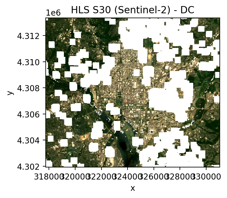
[7]:

# HLS S30 (Sentinel-2-derived, 30m)
try:
    data_hls_s30, df_hls_s30 = open_stac(
        stac_catalog='nasa_lp_cloud',
        collection='hls_s30',
        bounds=(-77.1, 38.85, -76.95, 38.95),
        epsg=32618,
        bands=['red', 'green', 'blue', 'nir'],
        start_date='2023-06-01',
        end_date='2023-07-31',
        cloud_cover_perc=30,
        resolution=30.0,
        max_items=3,
        mask_data=True,
    )

    print(f'HLS S30 shape: {data_hls_s30.shape}')
    print(f'Bands: {list(data_hls_s30.band.values)}')
    print(f'Times: {data_hls_s30.time.values}')

    fig, ax = plt.subplots(dpi=200, figsize=(4, 4))
    data_hls_s30.sel(
        time=data_hls_s30.time[0], band=['red', 'green', 'blue']
    ).plot.imshow(robust=True, ax=ax)
    ax.set_title('HLS S30 (Sentinel-2) - DC')
    ax.set_aspect('equal')
    plt.tight_layout(pad=1)
    plt.show()
except Exception as e:
    print(f'HLS S30 failed (need ~/.netrc credentials): {e}')

Searching nasa_lp_cloud for hls_s30...
Found 3 items.

Downloading hls_s30: 100%|██████████| 184/184 [00:30<00:00,  6.13it/s]

HLS S30 shape: (3, 4, 381, 443)
Bands: ['red', 'green', 'blue', 'nir']
Times: ['2023-06-02T16:12:23.667000000' '2023-06-07T16:12:23.236000000'
 '2023-06-29T16:02:28.946000000']

5. Cloud-Free Composites with `composite_stac()`#

composite_stac() wraps open_stac() to produce cloud-free temporal composites:

Searches STAC and loads imagery
Applies pixel-level cloud masking automatically
Groups by time period and takes the median (robust to outliers)
Preserves all spatial attributes for saving as GeoTIFF

The frequency parameter accepts pandas offset aliases:

Alias	Period
`'W'`	Weekly
`'MS'`	Monthly
`'QS'`	Quarterly
`'YS'`	Yearly

Sentinel-2 monthly composite#

[8]:

from geowombat.core.stac import composite_stac

# Monthly median composite - Sentinel-2
comp_s2, df_s2 = composite_stac(
    stac_catalog='element84_v1',
    collection='sentinel_s2_l2a',
    bounds=(-77.1, 38.85, -76.95, 38.95),
    epsg=32618,
    bands=['blue', 'green', 'red', 'nir'],
    start_date='2023-06-01',
    end_date='2023-08-31',
    cloud_cover_perc=50,
    resolution=100.0,
    chunksize=256,
    max_items=10,
    frequency='MS',
    compute=True,
)

print(f'Shape: {comp_s2.shape}')
print(f'Monthly timestamps: {comp_s2.time.values}')
print(f'Bands: {list(comp_s2.band.values)}')
print(f'NaN fraction: {float(np.isnan(comp_s2.values).mean()):.3f}')
print(f'CRS: {comp_s2.attrs["crs"]}, Res: {comp_s2.attrs["res"]}')

# Plot monthly composites
n_months = comp_s2.sizes['time']
fig, axes = plt.subplots(1, n_months, dpi=200, figsize=(5 * n_months, 5))
if n_months == 1:
    axes = [axes]
for i, ax in enumerate(axes):
    comp_s2.isel(time=i).sel(band=['red', 'green', 'blue']).plot.imshow(
        robust=True, ax=ax
    )
    month = str(comp_s2.time.values[i])[:7]
    ax.set_title(f'S2 Composite - {month}')
plt.tight_layout(pad=1)
plt.show()

Searching element84_v1 for sentinel_s2_l2a...
Found 10 items.

Downloading & compositing sentinel_s2_l2a: 100%|██████████| 245/245 [00:07<00:00, 33.74it/s]

Shape: (2, 4, 115, 134)
Monthly timestamps: ['2023-07-01T00:00:00.000000000' '2023-08-01T00:00:00.000000000']
Bands: ['blue', 'green', 'red', 'nir']
NaN fraction: 0.000
CRS: epsg:32618, Res: (100.0, 100.0)

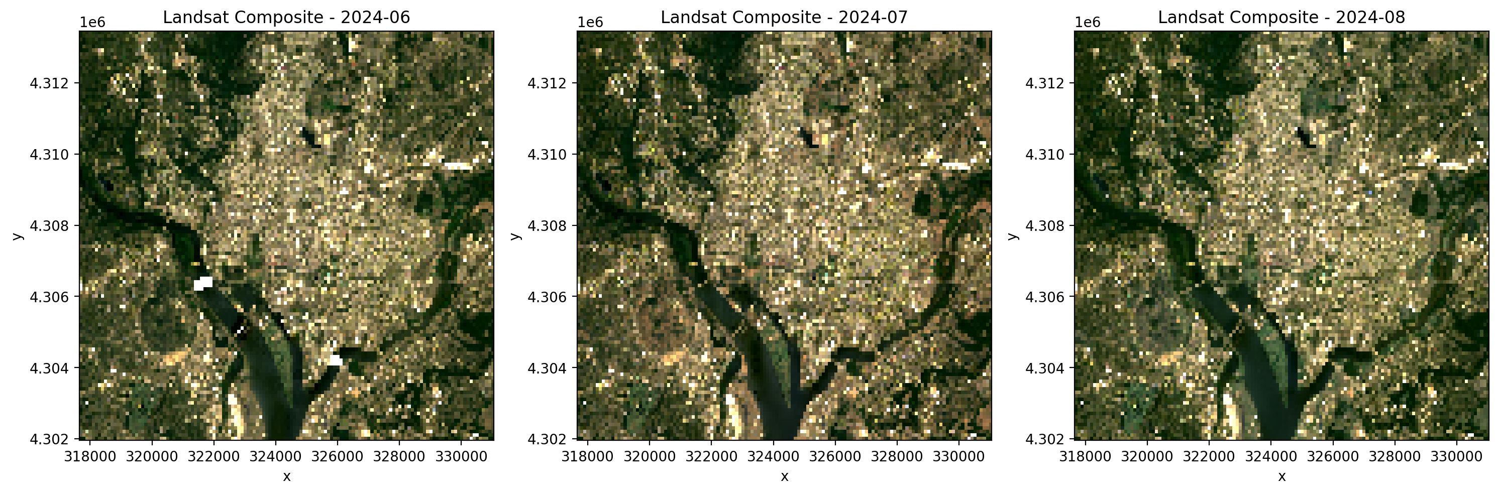
Landsat monthly composite#

[9]:

# Monthly median composite - Landsat
comp_ls, df_ls = composite_stac(
    stac_catalog='microsoft_v1',
    collection='landsat_c2_l2',
    bounds=(-77.1, 38.85, -76.95, 38.95),
    epsg=32618,
    bands=['red', 'green', 'blue'],
    start_date='2024-06-01',
    end_date='2024-08-31',
    cloud_cover_perc=50,
    resolution=100.0,
    chunksize=256,
    max_items=15,
    frequency='MS',
    compute=True,
)

print(f'Shape: {comp_ls.shape}')
print(f'Monthly timestamps: {comp_ls.time.values}')
print(f'Bands: {list(comp_ls.band.values)}')
print(f'NaN fraction: {float(np.isnan(comp_ls.values).mean()):.3f}')
print(f'CRS: {comp_ls.attrs["crs"]}, Res: {comp_ls.attrs["res"]}')

n_months = comp_ls.sizes['time']
fig, axes = plt.subplots(1, n_months, dpi=200, figsize=(5 * n_months, 5))
if n_months == 1:
    axes = [axes]
for i, ax in enumerate(axes):
    comp_ls.isel(time=i).plot.imshow(robust=True, ax=ax)
    month = str(comp_ls.time.values[i])[:7]
    ax.set_title(f'Landsat Composite - {month}')
plt.tight_layout(pad=1)
plt.show()

Searching microsoft_v1 for landsat_c2_l2...
Found 7 items.

Downloading & compositing landsat_c2_l2: 100%|██████████| 126/126 [00:03<00:00, 41.13it/s]

Shape: (3, 3, 115, 134)
Monthly timestamps: ['2024-06-01T00:00:00.000000000' '2024-07-01T00:00:00.000000000'
 '2024-08-01T00:00:00.000000000']
Bands: ['red', 'green', 'blue']
NaN fraction: 0.001
CRS: epsg:32618, Res: (100.0, 100.0)

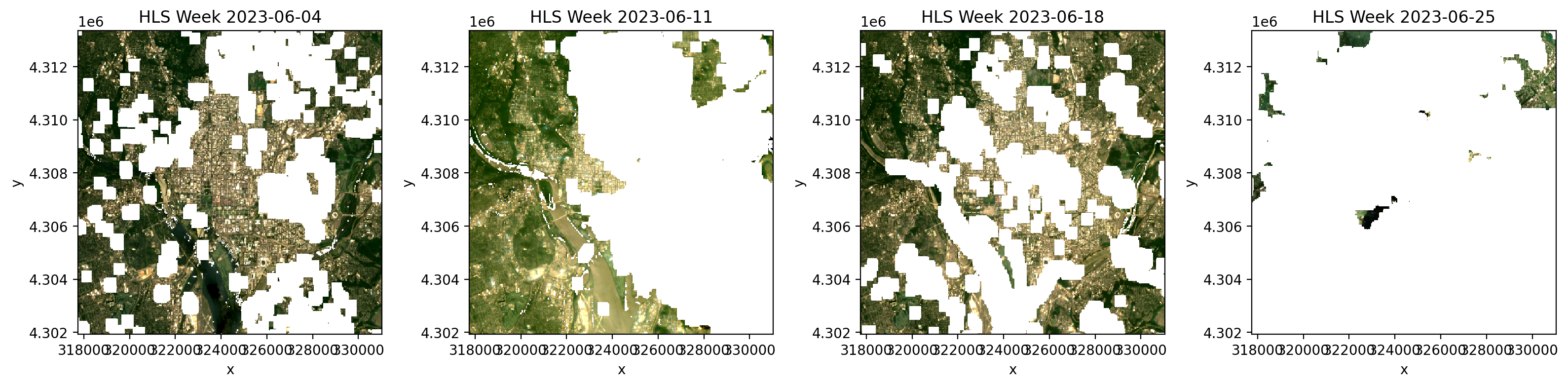
Combined HLS weekly composite#

Use collection='hls' to query both HLS L30 (Landsat) and S30 (Sentinel-2), merge observations from both sensors, and composite into cloud-free weekly mosaics. This maximizes temporal coverage (~3-day effective revisit) on a common 30m grid.

Note: Requires ~/.netrc with NASA Earthdata credentials.

[10]:

# Combined HLS (Landsat + Sentinel-2) weekly composite
try:
    comp_hls, df_hls = composite_stac(
        collection='hls',  # queries both hls_l30 and hls_s30
        bounds=(-77.1, 38.85, -76.95, 38.95),
        epsg=32618,
        bands=['red', 'green', 'blue', 'nir'],
        start_date='2023-06-01',
        end_date='2023-06-30',
        resolution=30,
        max_items=10,
        frequency='W',  # weekly composites
        compute=True,
    )

    print(f'Shape: {comp_hls.shape}')
    print(f'Weekly timestamps: {comp_hls.time.values}')
    print(f'Bands: {list(comp_hls.band.values)}')

    n_weeks = comp_hls.sizes['time']
    fig, axes = plt.subplots(
        1, min(n_weeks, 4), dpi=200, figsize=(4 * min(n_weeks, 4), 4)
    )
    if n_weeks == 1:
        axes = [axes]
    for i, ax in enumerate(axes[:4]):
        comp_hls.isel(time=i).sel(
            band=['red', 'green', 'blue']
        ).plot.imshow(robust=True, ax=ax)
        week = str(comp_hls.time.values[i])[:10]
        ax.set_title(f'HLS Week {week}')
    plt.tight_layout(pad=1)
    plt.show()
except Exception as e:
    print(f'HLS composite failed (need ~/.netrc credentials): {e}')

Searching nasa_lp_cloud for hls_l30...
Found 1 items.
Searching nasa_lp_cloud for hls_s30...
Found 10 items.

HLS L30 (Landsat): 100%|██████████| 62/62 [00:06<00:00,  9.77it/s]
HLS S30 (Sentinel-2): 100%|██████████| 611/611 [01:18<00:00,  7.78it/s]

Computing composite...
Shape: (5, 4, 381, 443)
Weekly timestamps: ['2023-06-04T00:00:00.000000000' '2023-06-11T00:00:00.000000000'
 '2023-06-18T00:00:00.000000000' '2023-06-25T00:00:00.000000000'
 '2023-07-02T00:00:00.000000000']
Bands: ['red', 'green', 'blue', 'nir']

6. Classification on STAC Data#

STAC data works directly with geowombat’s fit_predict() and all sklearn classifiers. For single-date images, use .isel(time=0) to get (band, y, x) shape. For multi-date, use temporal_mode to control how the time dimension is handled.

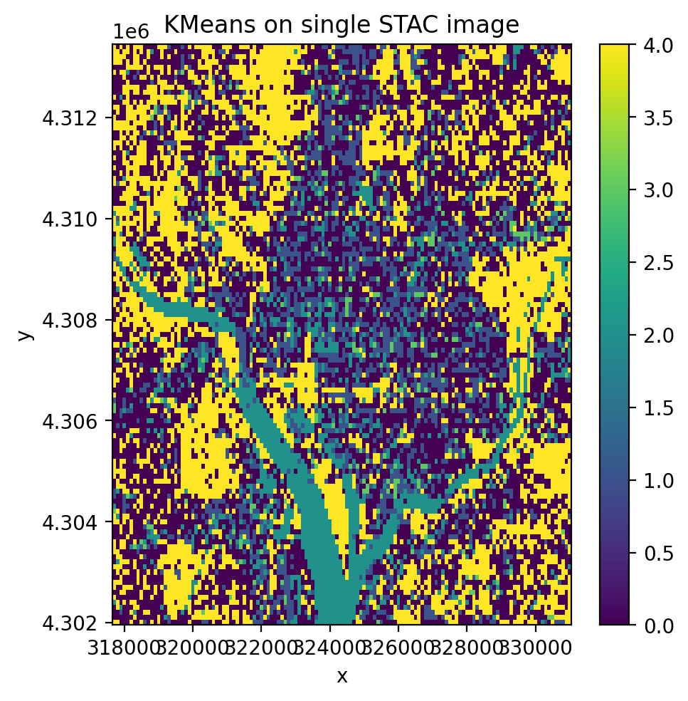
Unsupervised classification on a single STAC image#

[11]:

from sklearn.cluster import KMeans, MiniBatchKMeans
from sklearn.decomposition import PCA
from sklearn.pipeline import Pipeline
from sklearn.preprocessing import StandardScaler

from geowombat.ml import fit_predict

cl_stac = Pipeline(
    [('clf', MiniBatchKMeans(n_clusters=5, random_state=0))]
)

# Select a single time step and classify
single_image = data.isel(time=0)
print(f'Single image shape: {single_image.shape}')
print(f'Single image dims:  {single_image.dims}')

y_single = fit_predict(data=single_image, clf=cl_stac)

fig, ax = plt.subplots(dpi=200, figsize=(5, 5))
y_single.plot(robust=True, ax=ax)
ax.set_title('KMeans on single STAC image')
plt.tight_layout(pad=1)
plt.show()

Single image shape: (4, 115, 134)
Single image dims:  ('band', 'y', 'x')

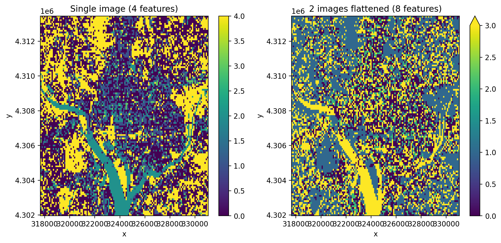
Multi-temporal classification with `temporal_mode='flatten'`#

Use all time steps as features. The T x B spectral-temporal features are flattened into a single band dimension, producing one classification map.

[12]:

cl_stac_flat = Pipeline([
    ('scaler', StandardScaler()),
    ('pca', PCA(n_components=2)),
    ('clf', KMeans(n_clusters=5, random_state=0)),
])

print(f'STAC data shape: {data.shape}  (time, band, y, x)')

y_stac_flat = fit_predict(
    data=data,
    clf=cl_stac_flat,
    temporal_mode='flatten',
)

print(f'Output shape:    {y_stac_flat.shape}  (no time dim)')
print(f'Output dims:     {y_stac_flat.dims}')

fig, axes = plt.subplots(1, 2, dpi=200, figsize=(10, 5))

y_single.plot(robust=True, ax=axes[0])
axes[0].set_title('Single image (4 features)')

y_stac_flat.plot(robust=True, ax=axes[1])
axes[1].set_title('2 images flattened (8 features)')

plt.tight_layout(pad=1)
plt.show()

STAC data shape: (1, 4, 115, 134)  (time, band, y, x)
Output shape:    (1, 115, 134)  (no time dim)
Output dims:     ('band', 'y', 'x')

Notes#

Saving results: y.gw.save('classification.tif', overwrite=True) or comp_s2.gw.save('composite.tif', overwrite=True)
``compute=True`` loads data into memory. Omit it to keep data lazy (dask-backed) for larger-than-memory workflows.
``chunksize`` controls the dask chunk size. Larger values use more memory but may be faster.
Deep learning on STAC data: See dl_classifiers.ipynb for TorchGeo pretrained models on STAC imagery.
Classical ML: See ml_classifiers.ipynb for supervised/unsupervised classification with bundled data.

Accessing Satellite Imagery with STAC

Contents