Accessing STAC Catalogs#

GeoWombat integrates easy access to Spatial Temporal Asset Catalog (STAC) APIs. STAC is a standardized way to expose collections of spatial temporal data. Instead of downloading large files, STAC lets you search for exactly the imagery you need (by location, date, and cloud cover) and stream it directly into your analysis. For a full list of public STAC APIs, refer to the STAC datasets page.

Installation#

To install geowombat with STAC functionality:

pip install "geowombat[stac]"

This installs the required dependencies: pystac, pystac_client, stackstac, and planetary_computer.

Supported catalogs and collections#

geowombat.core.stac.open_stac() supports the following STAC catalogs:

Catalog	Collections
`element84_v0`	`sentinel_s2_l2a_cogs`
`element84_v1`	`cop_dem_glo_30`, `landsat_c2_l2`, `sentinel_s2_l2a`, `sentinel_s2_l1c`, `sentinel_s1_l1c`, `naip`
`microsoft_v1`	`cop_dem_glo_30`, `landsat_c2_l1`, `landsat_c2_l2`, `landsat_l8_c2_l2`, `sentinel_s2_l2a`, `sentinel_s1_l1c`, `io_lulc`, `usda_cdl`, `esa_worldcover`
`nasa_lp_cloud`	`hls_l30` (HLS Landsat 30m), `hls_s30` (HLS Sentinel-2 30m)

STAC examples#

Stream Sentinel-2 data from Element 84#

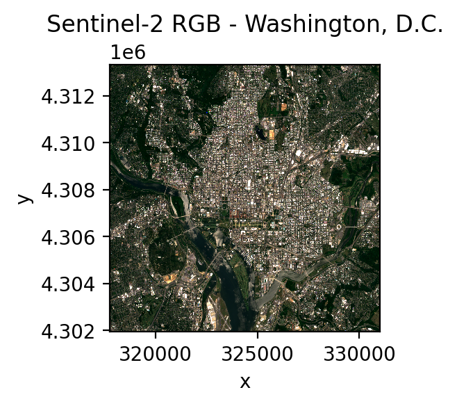
The following example streams Sentinel-2 Level 2A (surface reflectance) bands for the Washington, D.C. area using Element 84’s STAC catalog.

from geowombat.core.stac import open_stac

data, df = open_stac(
    stac_catalog="element84_v1",
    bounds=(-77.1, 38.85, -76.95, 38.95),  # DC area (left, bottom, right, top)
    epsg=32618,  # UTM Zone 18N
    collection="sentinel_s2_l2a",  # Sentinel-2 Level 2A (surface reflectance)
    bands=["blue", "green", "red", "nir"],
    cloud_cover_perc=20,
    start_date="2023-06-01",
    end_date="2023-07-31",
    resolution=10.0,
    chunksize=512,
)

# data is a lazy dask-backed xarray DataArray with dims (time, band, y, x)
print(data)

Plot the results:

import matplotlib.pyplot as plt

fig, ax = plt.subplots(dpi=200, figsize=(3, 3))
data.sel(time=data.time[0], band=["red", "green", "blue"]).plot.imshow(
    robust=True, ax=ax
)
ax.set_title("Sentinel-2 RGB - Washington, D.C.")
plt.tight_layout(pad=1)

Sentinel-2 RGB composite of Washington, D.C.

Stream Landsat data from Microsoft Planetary Computer#

from geowombat.core.stac import open_stac

data_l, df_l = open_stac(
    stac_catalog='microsoft_v1',
    collection='landsat_c2_l2',
    bounds=(-77.1, 38.85, -76.95, 38.95),
    epsg=32618,
    bands=['red', 'green', 'blue'],
    start_date='2023-06-01',
    end_date='2023-07-31',
    resolution=30.0,
    chunksize=512,
    max_items=5,
)

print(data_l)

fig, ax = plt.subplots(dpi=200, figsize=(3, 3))
data_l.sel(time=data_l.time[0]).plot.imshow(
    robust=True, ax=ax
)
ax.set_title("Landsat RGB - Washington, D.C.")
plt.tight_layout(pad=1)

Stream Harmonized Landsat Sentinel-2 (HLS) data from NASA#

HLS is a NASA product that provides BRDF-normalized surface reflectance from both Landsat OLI and Sentinel-2 MSI, resampled to a common 30m MGRS grid. This makes it straightforward to combine observations from both sensors into a single analysis-ready time series.

Two collections are available via the nasa_lp_cloud catalog:

``hls_l30`` — Landsat OLI (30m, ~8-day revisit)
``hls_s30`` — Sentinel-2 MSI (30m, ~5-day revisit)

You can use friendly band names (red, green, blue, nir, etc.) and GeoWombat automatically translates them to the correct HLS asset keys.

Common band names#
Name	L30 key	S30 key
`blue`	B02	B02
`green`	B03	B03
`red`	B04	B04
`nir`	B05	B8A
`swir1`	B06	B11
`swir2`	B07	B12

Authentication: HLS requires a free NASA Earthdata account. Create a ~/.netrc file with your credentials:

machine urs.earthdata.nasa.gov
login <your_username>
password <your_password>

Then set file permissions:

Linux/macOS: chmod 600 ~/.netrc
Windows: icacls %USERPROFILE%\.netrc /inheritance:r /grant:r %USERNAME%:R

from geowombat.core.stac import open_stac

# HLS Landsat 30m
data_l30, df = open_stac(
    stac_catalog="nasa_lp_cloud",
    collection="hls_l30",
    bounds=(-77.1, 38.85, -76.95, 38.95),
    epsg=32618,
    bands=["red", "green", "blue", "nir"],
    start_date="2023-06-01",
    end_date="2023-06-30",
    resolution=30.0,
    max_items=5,
)

# HLS Sentinel-2 30m
data_s30, df = open_stac(
    stac_catalog="nasa_lp_cloud",
    collection="hls_s30",
    bounds=(-77.1, 38.85, -76.95, 38.95),
    epsg=32618,
    bands=["red", "green", "blue", "nir"],
    start_date="2023-06-01",
    end_date="2023-06-30",
    resolution=30.0,
    max_items=5,
)

Tip

Use collection='hls' with composite_stac() to combine observations from both L30 and S30 into a single cloud-free composite. Only bands common to both sensors are allowed (blue, green, red, nir, swir1, swir2, coastal, cirrus). See the `Monthly composites`_ section below.

Cloud masking#

Set mask_data=True to automatically mask bad pixels. The appropriate QA band is auto-injected — you do not need to include qa_pixel or scl in your bands list.

Sentinel-2: Loads the SCL (Scene Classification Layer) band and masks clouds, cloud shadows, cirrus, saturated/defective pixels, and nodata. Default mask classes: no_data, saturated_defective, cloud_shadow, cloud_medium_prob, cloud_high_prob, thin_cirrus.
Landsat: Loads the qa_pixel band and applies a bitmask for fill, dilated cloud, cirrus, cloud, cloud shadow, and snow.
HLS: Loads the Fmask band and applies a bitmask for cirrus, cloud, adjacent cloud, cloud shadow, and snow/ice. Default mask classes: cirrus, cloud, adjacent_cloud, cloud_shadow, snow_ice.

# Sentinel-2 with cloud masking
data_s2, df = open_stac(
    stac_catalog="element84_v1",
    collection="sentinel_s2_l2a",
    bounds=(-77.1, 38.85, -76.95, 38.95),
    epsg=32618,
    bands=["blue", "green", "red", "nir"],
    start_date="2023-06-01",
    end_date="2023-07-31",
    cloud_cover_perc=50,
    resolution=100.0,
    max_items=5,
    mask_data=True,  # <-- auto-loads SCL, masks clouds
)

# Landsat with cloud masking
data_ls, df = open_stac(
    stac_catalog="microsoft_v1",
    collection="landsat_c2_l2",
    bounds=(-77.1, 38.85, -76.95, 38.95),
    epsg=32618,
    bands=["red", "green", "blue"],
    start_date="2023-06-01",
    end_date="2023-07-31",
    cloud_cover_perc=50,
    resolution=100.0,
    max_items=5,
    mask_data=True,  # <-- auto-loads qa_pixel, masks clouds
)

# HLS with cloud masking
data_hls, df = open_stac(
    stac_catalog="nasa_lp_cloud",
    collection="hls_l30",
    bounds=(-77.1, 38.85, -76.95, 38.95),
    epsg=32618,
    bands=["red", "green", "blue"],
    start_date="2023-06-01",
    end_date="2023-07-31",
    resolution=30.0,
    max_items=5,
    mask_data=True,  # <-- auto-loads Fmask, masks clouds
)

You can customize which classes are masked with the mask_items parameter:

# Only mask clouds and cloud shadow for Sentinel-2
data, df = open_stac(
    ...,
    collection="sentinel_s2_l2a",
    mask_data=True,
    mask_items=["cloud_shadow", "cloud_high_prob"],
)

# Only mask clouds and fill for Landsat
data, df = open_stac(
    ...,
    collection="landsat_c2_l2",
    mask_data=True,
    mask_items=["fill", "cloud", "cloud_shadow"],
)

# Only mask clouds for HLS
data, df = open_stac(
    ...,
    stac_catalog="nasa_lp_cloud",
    collection="hls_l30",
    mask_data=True,
    mask_items=["cloud", "cloud_shadow"],
)

Temporal composites#

Use geowombat.core.stac.composite_stac() to create cloud-free temporal composites. It wraps open_stac() with automatic cloud masking and temporal aggregation:

from geowombat.core.stac import composite_stac

# Monthly Sentinel-2 composite (median, the default)
comp_s2, df = composite_stac(
    stac_catalog="element84_v1",
    collection="sentinel_s2_l2a",
    bounds=(-77.1, 38.85, -76.95, 38.95),
    epsg=32618,
    bands=["blue", "green", "red", "nir"],
    start_date="2023-06-01",
    end_date="2023-08-31",
    cloud_cover_perc=50,
    resolution=100.0,
    max_items=20,
    frequency="MS",  # Monthly (default)
)

print(comp_s2.shape)  # (time=3, band=4, y, x) — one per month

Temporal frequency#

The frequency parameter accepts any pandas offset alias. Common values:

Alias	Description
`'D'`	Daily
`'W'`	Weekly
`'2W'`	Biweekly (every 2 weeks)
`'MS'`	Monthly — month start (default)
`'QS'`	Quarterly — quarter start
`'YS'`	Yearly — year start

Multiplied forms are supported: '15D' (every 15 days), '2MS' (every 2 months), etc.

Aggregation method#

The agg parameter controls how observations within each time period are combined. Default is 'median'.

Value	Description
`'median'`	Median (default) — robust to outliers
`'mean'`	Mean — sensitive to outliers
`'min'`	Minimum value per pixel
`'max'`	Maximum value per pixel

# Biweekly mean composite
comp, df = composite_stac(
    collection="sentinel_s2_l2a",
    bounds=(-77.1, 38.85, -76.95, 38.95),
    epsg=32618,
    bands=["blue", "green", "red", "nir"],
    start_date="2023-06-01",
    end_date="2023-08-31",
    resolution=10.0,
    frequency="2W",
    agg="mean",
)

# Quarterly Landsat composite
comp_ls, df = composite_stac(
    stac_catalog="microsoft_v1",
    collection="landsat_c2_l2",
    bounds=(-77.1, 38.85, -76.95, 38.95),
    epsg=32618,
    bands=["red", "green", "blue"],
    start_date="2023-01-01",
    end_date="2023-12-31",
    cloud_cover_perc=30,
    resolution=30.0,
    frequency="QS",
)

# Combined HLS (Landsat + Sentinel-2) monthly composite
comp_hls, df = composite_stac(
    collection="hls",  # queries both hls_l30 and hls_s30
    bounds=(-77.1, 38.85, -76.95, 38.95),
    epsg=32618,
    bands=["blue", "green", "red", "nir"],
    start_date="2023-06-01",
    end_date="2023-08-31",
    resolution=30.0,
    frequency="MS",
    max_items=20,
)

print(comp_hls.shape)  # more observations per period from two sensors

Note

Composites preserve all spatial attributes (crs, res, transform) so you can save directly with gw.save(). Time periods where all pixels are cloudy are automatically dropped from the output.

Merge multiple collections#

Use geowombat.core.stac.merge_stac() to combine data from different sensors into a single time series:

from geowombat.core.stac import open_stac, merge_stac
from rasterio.enums import Resampling

# Load Landsat
data_l, df_l = open_stac(
    stac_catalog="microsoft_v1",
    collection="landsat_c2_l2",
    bounds=(-77.1, 38.85, -76.95, 38.95),
    bands=["red", "green", "blue"],
    mask_data=True,
    start_date="2023-01-01",
    end_date="2023-12-31",
    epsg=32618,
    resolution=30.0,
)

# Load Sentinel-2, reprojected to match Landsat
data_s2, df_s2 = open_stac(
    stac_catalog="element84_v1",
    collection="sentinel_s2_l2a",
    bounds=(-77.1, 38.85, -76.95, 38.95),
    bands=["blue", "green", "red"],
    resampling=Resampling.cubic,
    epsg=32618,
    start_date="2023-01-01",
    end_date="2023-12-31",
    resolution=30.0,
)

# Merge into a single time series
stack = merge_stac(data_l, data_s2)
print(stack)