Deep Learning Classifiers in GeoWombat#
This notebook demonstrates how to use GeoWombat’s deep learning classifiers for land cover classification using the same fit() / predict() / fit_predict() API as the classical ML classifiers.
Requirements: pip install geowombat[dl]
This installs: torch, pytorch-tabnet, torchgeo, segmentation-models-pytorch
Setup#
[1]:
import os
os.environ['CPL_LOG'] = '/dev/null'  # suppress GDAL warnings

import warnings
warnings.filterwarnings('ignore')

import matplotlib.pyplot as plt
import geopandas as gpd
import numpy as np

import geowombat as gw
from geowombat.data import (
    l8_224078_20200518,
    stac_training,
)
from geowombat.ml import fit, fit_predict, predict
Prepare training labels#
Load the training polygons bundled in geowombat.data. The lc column contains integer land cover class labels (already encoded).
[2]:
# Load training polygons (integer 'lc' column, EPSG:4326)
labels = gpd.read_file(stac_training)
print(f"Labels shape: {labels.shape}")
print(f"CRS: {labels.crs}")
print(f"Classes: {sorted(labels['lc'].unique())}")
print(f"Number of classes: {labels['lc'].nunique()}")
labels.head()
Labels shape: (7, 3)
CRS: EPSG:4326
Classes: [0, 1, 2, 3, 5]
Number of classes: 5
[2]:
| fid | lc | geometry | |
|---|---|---|---|
| 0 | 1 | 0 | POLYGON ((-54.64919 -25.25946, -54.64925 -25.2... |
| 1 | 2 | 0 | POLYGON ((-54.62817 -25.27092, -54.62803 -25.2... |
| 2 | 3 | 2 | POLYGON ((-54.6147 -25.27095, -54.60949 -25.26... |
| 3 | 4 | 1 | POLYGON ((-54.61715 -25.28278, -54.62002 -25.2... |
| 4 | 5 | 1 | POLYGON ((-54.58943 -25.32398, -54.58966 -25.3... |
Preview the image and labels#
[3]:
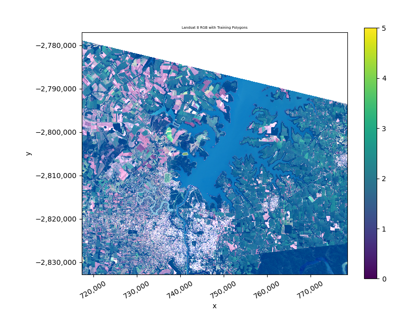
with gw.open(l8_224078_20200518, nodata=0) as src:
    print(f"Image shape: {src.shape}")
    print(f"Image dims:  {src.dims}")
    print(f"CRS:         {src.crs}")
    print(f"Resolution:  {src.res}")

    fig, ax = plt.subplots(1, 1, figsize=(8, 6))
    src.sel(band=[3, 2, 1]).gw.imshow(mask=True, nodata=0, robust=True, ax=ax)
    labels.to_crs(src.crs).plot(
        ax=ax, column='lc', legend=True,
        edgecolor='white', linewidth=1, alpha=0.5,
    )
    ax.set_title('Landsat 8 RGB with Training Polygons')
    ax.set_aspect('equal')
    plt.tight_layout()
    plt.show()
Image shape: (3, 1860, 2041)
Image dims:  ('band', 'y', 'x')
CRS:         32621
Resolution:  (30.0, 30.0)
1. TabNet Classifier#
TabNet is an attention-based tabular deep learning model. In GeoWombat, each pixel is treated as a sample with spectral bands as features (pixel-wise classification).
Key parameters:
max_epochs: Number of training epochsbatch_size: Mini-batch size (default 1024)patience: Early stopping patience (default 10)verbose: 0=silent, 1=progressdevice: ‘cpu’, ‘cuda’, or ‘auto’
1a. TabNet with fit_predict() (one-step)#
[4]:
from geowombat.ml.dl_classifiers import TabNetClassifier

with gw.config.update(ref_res=150):
    with gw.open(l8_224078_20200518, nodata=0) as src:
        # One-step: fit and predict in a single call
        y = fit_predict(
            src,
            TabNetClassifier(max_epochs=50, verbose=0),
            labels,
            col='lc',
        )

print(f"Prediction shape: {y.shape}")
print(f"Prediction dims:  {y.dims}")
print(f"Unique values:    {np.unique(y.values[np.isfinite(y.values)])}")
Prediction shape: (372, 408, 1)
Prediction dims:  ('y', 'x', 'band')
Unique values:    [1. 2. 3. 4. 5.]
[5]:
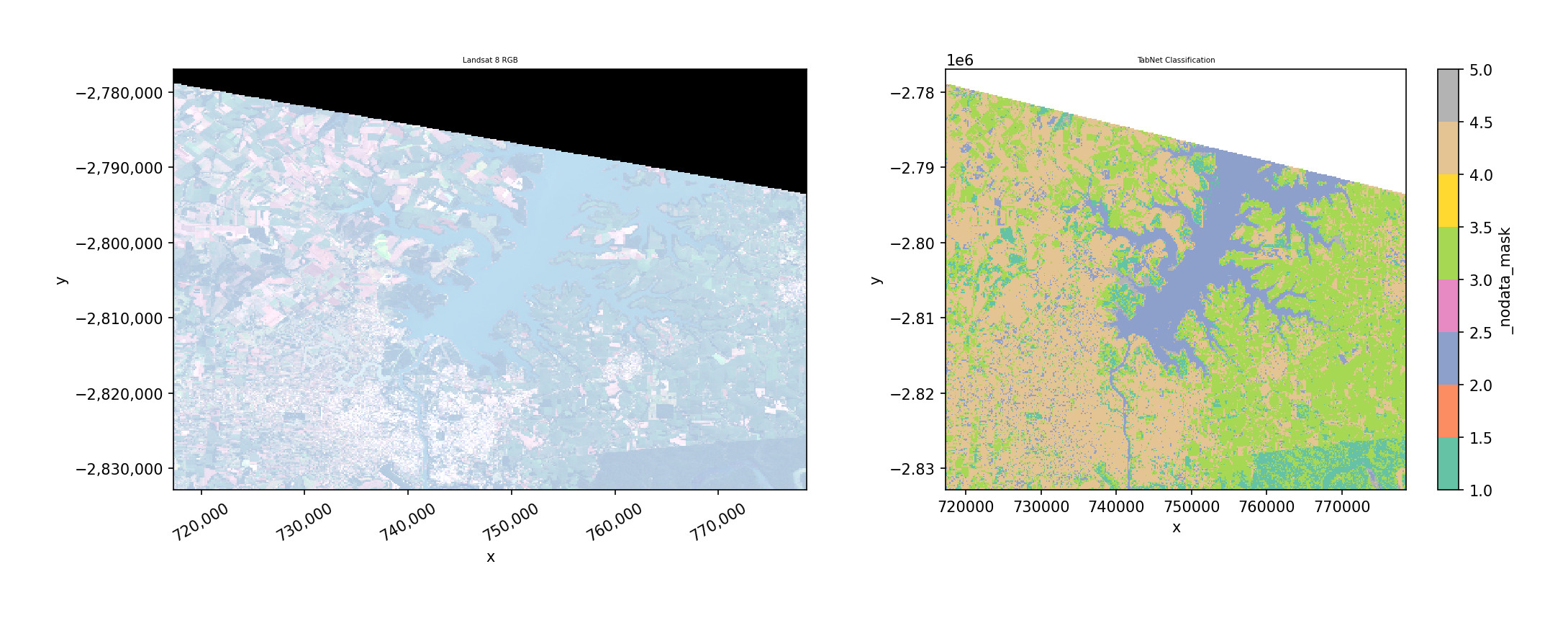
# Plot the TabNet classification result
fig, axes = plt.subplots(1, 2, figsize=(14, 5))

with gw.config.update(ref_res=150):
    with gw.open(l8_224078_20200518, nodata=0) as src:
        src.sel(band=[3, 2, 1]).gw.imshow(mask=True, nodata=0, robust=True, ax=axes[0])
        axes[0].set_title('Landsat 8 RGB')

y.sel(band='targ').plot(ax=axes[1], cmap='Set2', add_colorbar=True)
axes[1].set_title('TabNet Classification')
axes[1].set_aspect('equal')

plt.tight_layout()
plt.show()
1b. TabNet with separate fit() then predict()#
Use separate steps when you want to inspect the trained model, save it, or predict on different data.
[6]:
with gw.config.update(ref_res=150):
    with gw.open(l8_224078_20200518, nodata=0) as src:
        # Step 1: Fit the model
        clf = TabNetClassifier(max_epochs=50, verbose=0)
        X, Xy, clf = fit(src, clf, labels, col='lc')

        print(f"Model fitted: {clf.fitted_}")
        print(f"Number of classes: {clf._n_classes}")

        # Step 2: Predict (can use same or different data)
        y = predict(src, X, clf)

print(f"\nPrediction shape: {y.shape}")
vals = y.values[np.isfinite(y.values)]
print(f"Unique predictions: {np.unique(vals)}")
Model fitted: True
Number of classes: 5

Prediction shape: (372, 408, 1)
Unique predictions: [1. 2. 3. 4. 5.]
2. L-TAE Classifier (Temporal Attention)#
The Lightweight Temporal Attention Encoder (L-TAE) is designed for satellite image time series. It uses multi-head temporal attention to classify each pixel based on its spectral trajectory across multiple dates.
Key requirement: Data must have a time dimension (opened with stack_dim='time').
Key parameters:
n_head: Number of attention heads (default 4)d_k: Key dimension per head (default 32)d_model: Internal embedding dimension (default 128)max_epochs: Training epochslr: Learning rate (default 1e-3)device: ‘cpu’, ‘cuda’, or ‘auto’
2a. Open multi-temporal data#
L-TAE requires time-stacked data. Here we stack the same image twice to simulate a 2-date time series (in practice, use different acquisition dates).
[7]:
from geowombat.ml.dl_classifiers import LTAEClassifier

with gw.config.update(ref_res=150):
    with gw.open(
        [l8_224078_20200518, l8_224078_20200518],
        stack_dim='time',
        nodata=0,
    ) as src:
        print(f"Multi-temporal shape: {src.shape}")
        print(f"Dims: {src.dims}")
        print(f"Time steps: {src.sizes['time']}")
        print(f"Bands: {src.sizes['band']}")
Multi-temporal shape: (2, 3, 372, 408)
Dims: ('time', 'band', 'y', 'x')
Time steps: 2
Bands: 3
2b. L-TAE with fit_predict()#
[8]:
with gw.config.update(ref_res=150):
    with gw.open(
        [l8_224078_20200518, l8_224078_20200518],
        stack_dim='time',
        nodata=0,
    ) as src:
        y = fit_predict(
            src,
            LTAEClassifier(
                max_epochs=50,
                verbose=0,
                d_model=32,   # smaller model for demo
                d_k=8,
                n_head=2,
            ),
            labels,
            col='lc',
        )

print(f"Prediction shape: {y.shape}")
print(f"Prediction dims:  {y.dims}")
print(f"Unique values:    {np.unique(y.values[np.isfinite(y.values)])}")
Prediction shape: (372, 408, 1)
Prediction dims:  ('y', 'x', 'band')
Unique values:    [2. 3. 4. 5.]
[9]:
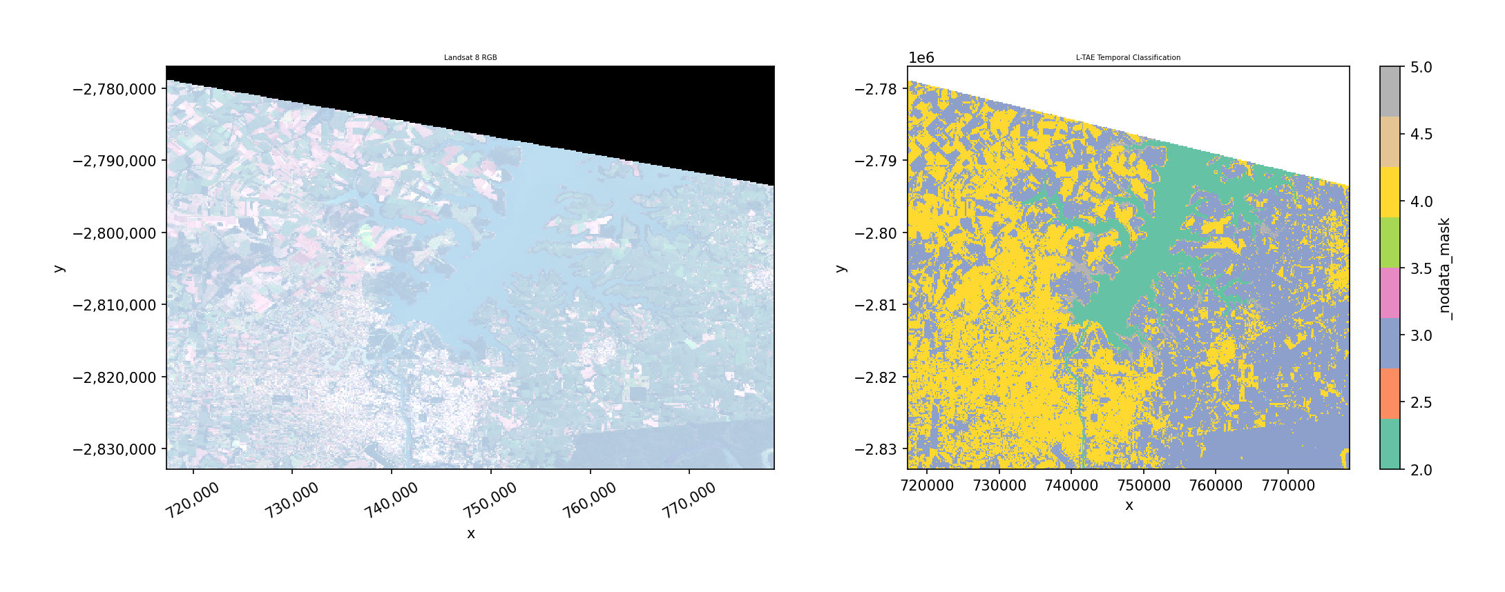
# Plot the L-TAE classification result
fig, axes = plt.subplots(1, 2, figsize=(14, 5))

with gw.config.update(ref_res=150):
    with gw.open(l8_224078_20200518, nodata=0) as src:
        src.sel(band=[3, 2, 1]).gw.imshow(mask=True, nodata=0, robust=True, ax=axes[0])
        axes[0].set_title('Landsat 8 RGB')

y.sel(band='targ').plot(ax=axes[1], cmap='Set2', add_colorbar=True)
axes[1].set_title('L-TAE Temporal Classification')
axes[1].set_aspect('equal')

plt.tight_layout()
plt.show()
2c. L-TAE with separate fit() then predict()#
[10]:
with gw.config.update(ref_res=150):
    with gw.open(
        [l8_224078_20200518, l8_224078_20200518],
        stack_dim='time',
        nodata=0,
    ) as src:
        # Step 1: Fit
        clf = LTAEClassifier(
            max_epochs=50,
            verbose=0,
            d_model=32,
            d_k=8,
            n_head=2,
        )
        X, Xy, clf = fit(src, clf, labels, col='lc')

        print(f"Model fitted: {clf.fitted_}")
        print(f"Classes: {clf._n_classes}")
        print(f"Bands: {clf._n_bands}, Timesteps: {clf._n_timesteps}")

        # Step 2: Predict
        y = predict(src, X, clf)

print(f"\nPrediction shape: {y.shape}")
vals = y.values[np.isfinite(y.values)]
print(f"Unique predictions: {np.unique(vals)}")
Model fitted: True
Classes: 5
Bands: 3, Timesteps: 2

Prediction shape: (372, 408, 1)
Unique predictions: [2. 3. 4. 5.]
2d. L-TAE error handling: no time dimension#
L-TAE raises a clear error if data doesn’t have a time dimension.
[11]:
# This will raise a ValueError
try:
    with gw.config.update(ref_res=150):
        with gw.open(l8_224078_20200518, nodata=0) as src:
            clf = LTAEClassifier()
            fit(src, clf, labels, col='lc')
except ValueError as e:
    print(f"Expected error: {e}")
Expected error: LTAEClassifier requires multi-temporal data with a 'time' dimension. Open data with stack_dim='time'.
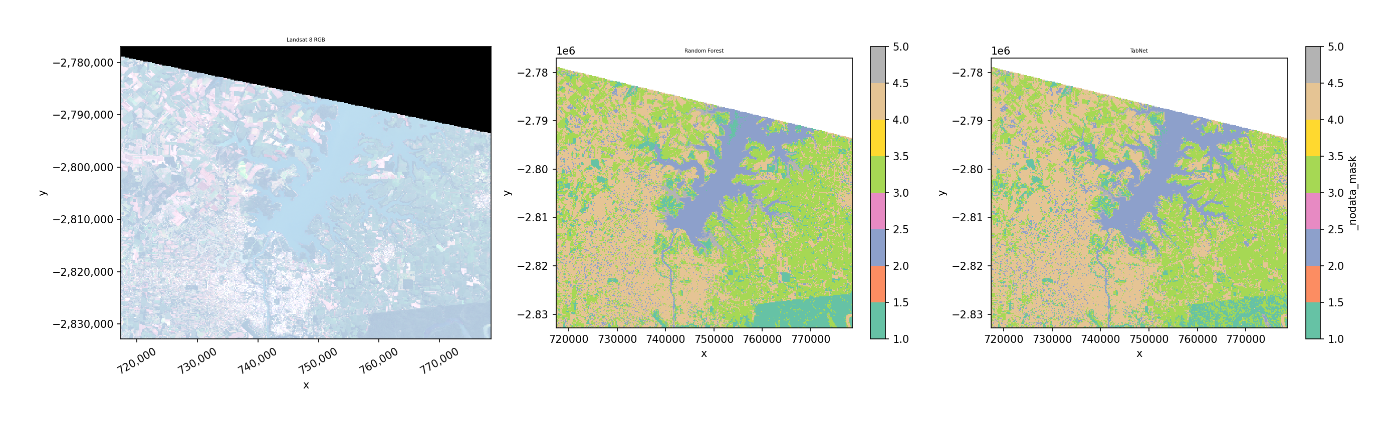
3. Comparison with Classical ML#
The DL classifiers use the exact same fit() / predict() / fit_predict() API as sklearn-based classifiers. Here’s a side-by-side comparison.
[12]:
from sklearn.ensemble import RandomForestClassifier

with gw.config.update(ref_res=150):
    with gw.open(l8_224078_20200518, nodata=0) as src:
        # Classical ML: Random Forest
        y_rf = fit_predict(
            src,
            RandomForestClassifier(n_estimators=50, random_state=42),
            labels,
            col='lc',
        )

        # Deep Learning: TabNet
        y_tabnet = fit_predict(
            src,
            TabNetClassifier(max_epochs=50, verbose=0),
            labels,
            col='lc',
        )

# Plot side by side
fig, axes = plt.subplots(1, 3, figsize=(18, 5))

with gw.config.update(ref_res=150):
    with gw.open(l8_224078_20200518, nodata=0) as src:
        src.sel(band=[3, 2, 1]).gw.imshow(mask=True, nodata=0, robust=True, ax=axes[0])
        axes[0].set_title('Landsat 8 RGB')

y_rf.sel(band='targ').plot(ax=axes[1], cmap='Set2', add_colorbar=True)
axes[1].set_title('Random Forest')
axes[1].set_aspect('equal')

y_tabnet.sel(band='targ').plot(ax=axes[2], cmap='Set2', add_colorbar=True)
axes[2].set_title('TabNet')
axes[2].set_aspect('equal')

plt.tight_layout()
plt.show()
4. TorchGeo Pretrained Model Reference#
TorchGeo provides 60+ pretrained encoder weights for satellite-specific feature extraction. These can be used with TorchGeoClassifier(backbone=..., weights='...') to leverage encoders pre-trained on satellite imagery (Sentinel-2, Landsat, NAIP, etc.).
The table below is generated programmatically — it auto-updates as TorchGeo adds new weights.
[13]:
import torchgeo.models
import enum
import pandas as pd

rows = []
for attr_name in sorted(dir(torchgeo.models)):
    obj = getattr(torchgeo.models, attr_name)
    if not attr_name.endswith('_Weights'):
        continue
    if not (isinstance(obj, type) and issubclass(obj, enum.Enum)):
        continue
    backbone = attr_name.replace('_Weights', '')
    for member in obj:
        meta = member.meta if hasattr(member, 'meta') else {}
        rows.append({
            'Backbone': backbone,
            'Weight': f'{attr_name}.{member.name}',
            'Sensor': meta.get('dataset', ''),
            'In Channels': meta.get('in_chans', ''),
            'Bands': ', '.join(meta.get('bands', [])),
        })

df = pd.DataFrame(rows)
print(f"Total pretrained weights available: {len(df)}")
df.sort_values(['In Channels', 'Backbone']).reset_index(drop=True)
Total pretrained weights available: 124
[13]:
| Backbone | Weight | Sensor | In Channels | Bands | |
|---|---|---|---|---|---|
| 0 | ResNet50 | ResNet50_Weights.SENTINEL1_ALL_DECUR | SSL4EO-S12 | 2 | VV, VH |
| 1 | ResNet50 | ResNet50_Weights.SENTINEL1_ALL_MOCO | SSL4EO-S12 | 2 | VV, VH |
| 2 | ResNet50 | ResNet50_Weights.SENTINEL1_GRD_CLOSP | CrisisLandMark | 2 | VV, VH |
| 3 | ResNet50 | ResNet50_Weights.SENTINEL1_GRD_GEOCLOSP | CrisisLandMark | 2 | VV, VH |
| 4 | ResNet50 | ResNet50_Weights.SENTINEL1_GRD_SOFTCON | SSL4EO-S12 | 2 | VV, VH |
| ... | ... | ... | ... | ... | ... |
| 119 | CROMALarge | CROMALarge_Weights.CROMA_VIT | SSL4EO | ||
| 120 | CopernicusFM_Base | CopernicusFM_Base_Weights.CopernicusFM_ViT | Copernicus-Pretrain | ||
| 121 | DOFABase16 | DOFABase16_Weights.DOFA_MAE | SatlasPretrain, Five-Billion-Pixels, HySpecNet... | ||
| 122 | DOFALarge16 | DOFALarge16_Weights.DOFA_MAE | SatlasPretrain, Five-Billion-Pixels, HySpecNet... | ||
| 123 | Panopticon | Panopticon_Weights.VIT_BASE14 |
124 rows × 5 columns
5. STAC + TorchGeo Pretrained Model Example#
Download Sentinel-2 imagery from a STAC catalog over the same area as our bundled Landsat data, then classify it using a TorchGeo U-Net with a pretrained encoder.
Requirements: pip install geowombat[stac] and network access.
We use composite_stac() to create a cloud-free median composite, which automatically handles cloud masking using the Sentinel-2 SCL band. Training labels are loaded from stac_training.geojson (bundled in geowombat.data), which has a lc column with integer class labels in EPSG:4326.
[14]:
from geowombat.core.stac import composite_stac
from geowombat.ml.dl_classifiers import TorchGeoClassifier

# Create a cloud-free Sentinel-2 RGB composite over the Landsat test area
# composite_stac() auto-masks clouds using the SCL band and takes the median
try:
    data, metadata = composite_stac(
        stac_catalog="element84_v1",
        collection="sentinel_s2_l2a",
        bounds=(-54.65, -25.41, -54.58, -25.25),
        epsg=32621,
        bands=["red", "green", "blue"],
        start_date="2023-06-01",
        end_date="2023-12-31",
        cloud_cover_perc=30,
        resolution=100.0,
        frequency="YS",       # yearly composite
        agg="median",          # median pixel value
        max_items=10,
        compute=True,
    )
    # composite_stac returns (time, band, y, x); take the single composite
    img = data.isel(time=0) if 'time' in data.dims else data
    print(f"Composite shape: {img.shape}")
    print(f"Dims: {img.dims}")
    STAC_OK = True
except Exception as e:
    print(f"STAC download failed (need network): {e}")
    print("Skipping STAC examples.")
    STAC_OK = False
Searching element84_v1 for sentinel_s2_l2a...
Found 10 items.
Downloading & compositing sentinel_s2_l2a: 100%|██████████| 162/162 [00:04<00:00, 39.04it/s]
Composite shape: (3, 179, 75)
Dims: ('band', 'y', 'x')
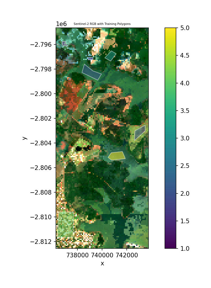
[15]:
# Plot the downloaded Sentinel-2 image with training polygons
if STAC_OK:
    fig, ax = plt.subplots(1, 1, figsize=(8, 6))
    img.plot.imshow(robust=True, ax=ax)
    labels.to_crs(img.attrs.get('crs', labels.crs)).plot(
        ax=ax, column='lc', legend=True,
        edgecolor='white', linewidth=1, alpha=0.5,
    )
    ax.set_title('Sentinel-2 RGB with Training Polygons')
    ax.set_aspect('equal')
    plt.tight_layout()
    plt.show()
else:
    print("Skipped — no STAC data available.")
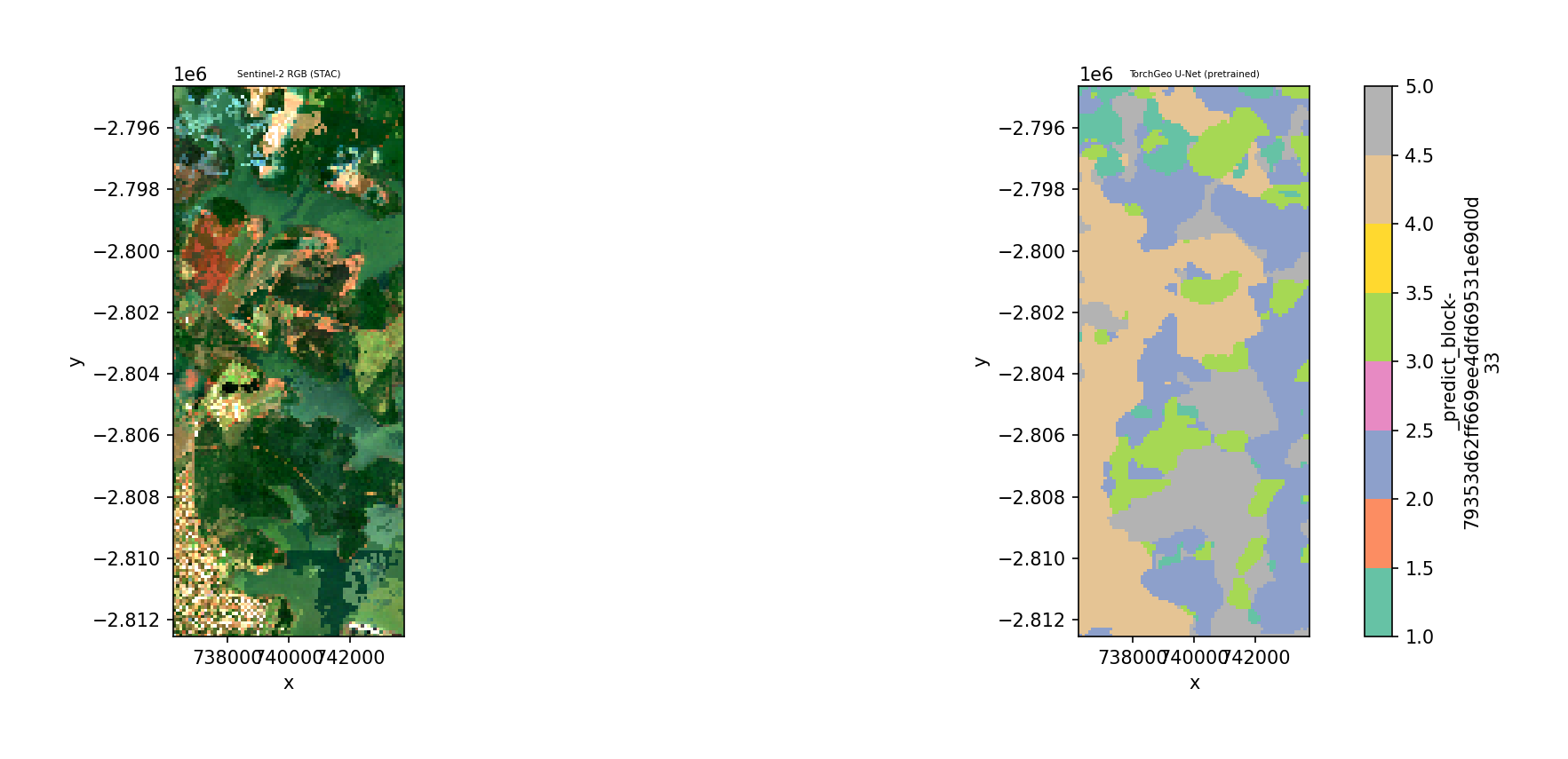
[16]:
# Classify the Sentinel-2 image using a pretrained TorchGeo U-Net
if STAC_OK:
    clf = TorchGeoClassifier(
        model='unet',
        backbone='resnet18',
        weights='ResNet18_Weights.SENTINEL2_RGB_MOCO',
        patch_size=32,
        max_epochs=5,
        batch_size=4,
        verbose=0,
    )
    y_stac = fit_predict(img, clf, labels, col='lc')

    print(f"Prediction shape: {y_stac.shape}")
    print(f"Unique values: {np.unique(y_stac.values[np.isfinite(y_stac.values)])}")
else:
    print("Skipped — no STAC data available.")
Prediction shape: (1, 179, 75)
Unique values: [1. 2. 3. 4. 5.]
[17]:
# Plot STAC classification result
if STAC_OK:
    fig, axes = plt.subplots(1, 2, figsize=(14, 5))
    img.plot.imshow(robust=True, ax=axes[0])
    axes[0].set_title('Sentinel-2 RGB (STAC)')
    axes[0].set_aspect("equal")

    y_stac.sel(band='targ').plot(ax=axes[1], cmap='Set2', add_colorbar=True)
    axes[1].set_title('TorchGeo U-Net (pretrained)')
    axes[1].set_aspect('equal')

    plt.tight_layout()
    plt.show()
else:
    print("Skipped — no STAC data available.")
Notes#
``n_classes`` is auto-inferred from the label column during
fit(). You never need to specify it.Feature normalization is handled internally — raw DN values are standardized before training/prediction.
Labels use 1-based encoding internally (0 = nodata). The classifiers handle the conversion to 0-based for PyTorch and back.
``ref_res`` controls the output resolution. Use a coarser resolution (e.g., 150-300m) for faster demos.
Device: Pass
device='cuda'ordevice='auto'to use GPU acceleration.For real workflows, increase
max_epochs(e.g., 50-200) and use full resolution data.L-TAE is most useful with real multi-date imagery where temporal patterns differ between classes.
This demo uses the same image stacked twice for L-TAE — in practice, use imagery from different dates.
The pretrained weights table (Section 4) auto-updates when TorchGeo adds new models.
STAC examples (Section 5) require network access; they are skipped gracefully if offline.