Mosaicing Tiles and Basic Calculations

This notebook illustrates the use of opening, mosaicing, band math, and masking.

Start

# %load_ext watermark

import geowombat as gw
from geowombat.data import rgbn_suba, rgbn_subb

%watermark -a "GeoWombat examples" -d -v -m -p dask,geowombat,numpy,rasterio,xarray -g

GeoWombat examples 2020-03-15

CPython 3.7.5
IPython 7.12.0

dask 2.11.0
geowombat 1.2.6
numpy 1.18.1
rasterio 1.1.3
xarray 0.15.0

compiler   : GCC 8.3.0
system     : Linux
release    : 4.15.0-88-generic
machine    : x86_64
processor  : x86_64
CPU cores  : 8
interpreter: 64bit
Git hash   : b62c1060763de9c5902082cd01e478b15469ae33

Opening files

Files are opened lazily using xarray.open_rasterio as a backend. This means that the data structure is setup as an xarray.DataArray with an underlying dask array, but data are not loaded upon opening.

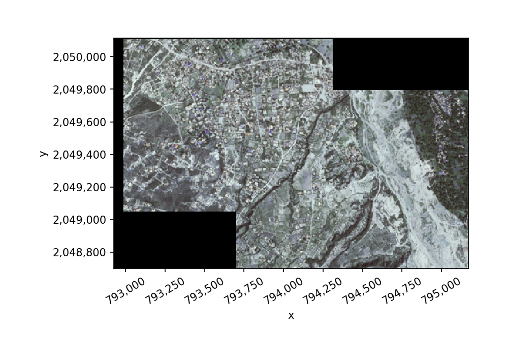
Image mosaicking

Mosaic the two subsets into a single DataArray. If the images in the mosaic list have the same CRS, no configuration is needed.

with gw.open([rgbn_suba, rgbn_subb],
              band_names=['blue', 'green', 'red', 'nir'],
              mosaic=True,
              bounds_by='union') as ds_mos:
     print(ds_mos)

<xarray.DataArray (band: 4, y: 283, x: 449)>
dask.array<maximum, shape=(4, 283, 449), dtype=uint8, chunksize=(1, 64, 64), chunktype=numpy.ndarray>
Coordinates:
  * band     (band) <U5 'blue' 'green' 'red' 'nir'
  * y        (y) float64 2.05e+06 2.05e+06 2.05e+06 ... 2.049e+06 2.049e+06
  * x        (x) float64 7.929e+05 7.929e+05 7.929e+05 ... 7.952e+05 7.952e+05
Attributes:
    transform:   (5.0, 0.0, 792925.0, 0.0, -5.0, 2050115.0)
    crs:         +init=epsg:32618
    res:         (5.0, 5.0)
    is_tiled:    0
    nodatavals:  (0.0, 0.0, 0.0, 0.0)
    scales:      (1.0, 1.0, 1.0, 1.0)
    offsets:     (0.0, 0.0, 0.0, 0.0)
    resampling:  nearest

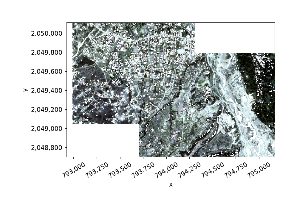
Plotting

Array plotting DataArray.plot.imshow() or DataArray.gw.imshow(). The latter is just a wrapper around the former to tidy up the plot axes. Note that only 1- or 3-band arrays can be plotted

ds_mos.sel(band=['blue', 'green', 'red']).gw.imshow()

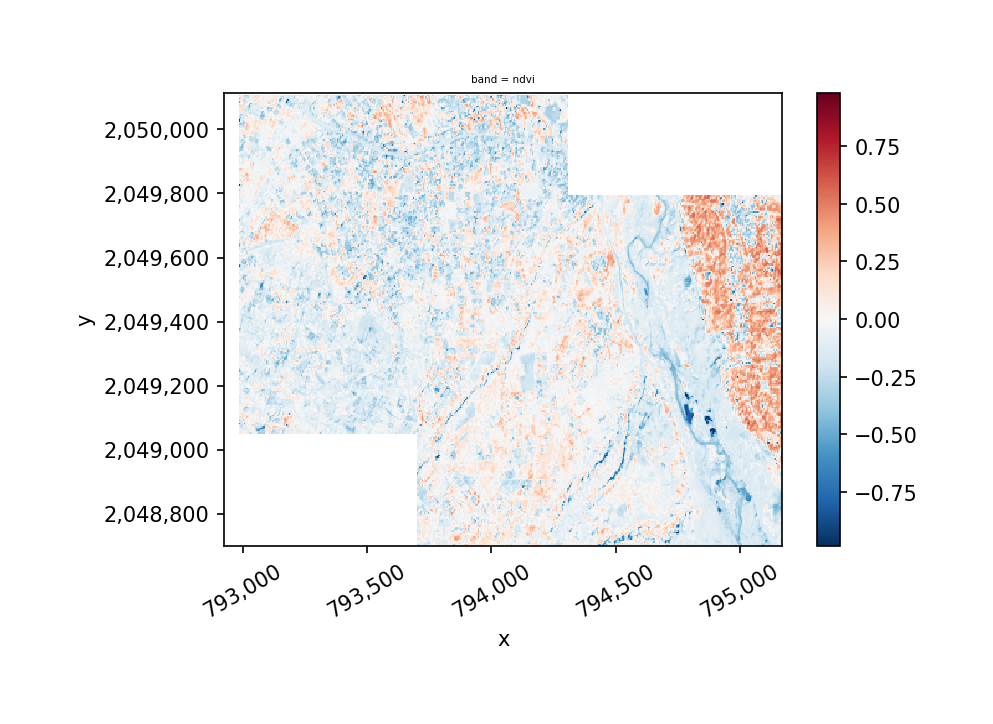
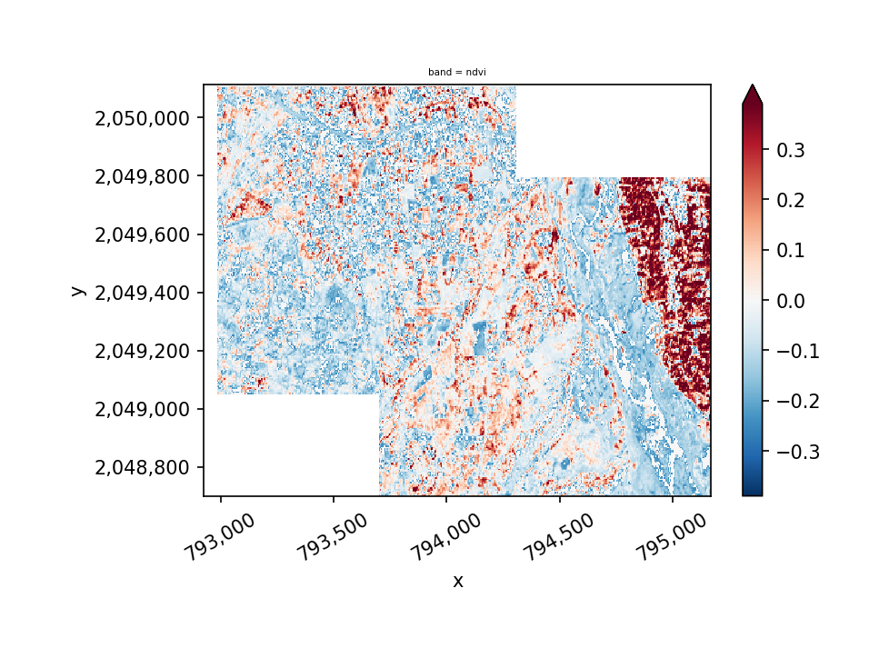
Calculating NDVI

Now let’s calculate NDVI. In order to do this we need to update our sensor configuration to take into account the band types and the scale factor for the data.

with gw.config.update(sensor='bgrn', scale_factor=0.0001):
    with gw.open([rgbn_suba, rgbn_subb],
          mosaic=True,
          bounds_by='union') as ds_mos:

              # calculate NDVI
              ndvi = ds_mos.gw.ndvi()
              print(ndvi)

ndvi.sel(band='ndvi').gw.imshow()

<xarray.DataArray (band: 1, y: 283, x: 449)>
dask.array<broadcast_to, shape=(1, 283, 449), dtype=float64, chunksize=(1, 64, 64), chunktype=numpy.ndarray>
Coordinates:
  * y        (y) float64 2.05e+06 2.05e+06 2.05e+06 ... 2.049e+06 2.049e+06
  * x        (x) float64 7.929e+05 7.929e+05 7.929e+05 ... 7.952e+05 7.952e+05
  * band     (band) <U4 'ndvi'
Attributes:
    transform:    (5.0, 0.0, 792925.0, 0.0, -5.0, 2050115.0)
    crs:          +init=epsg:32618
    res:          (5.0, 5.0)
    is_tiled:     0
    nodatavals:   None
    scales:       1.0
    offsets:      0.0
    sensor:       bgrn
    resampling:   nearest
    pre-scaling:  0.0001
    vi:           ndvi
    drange:       (-1, 1)

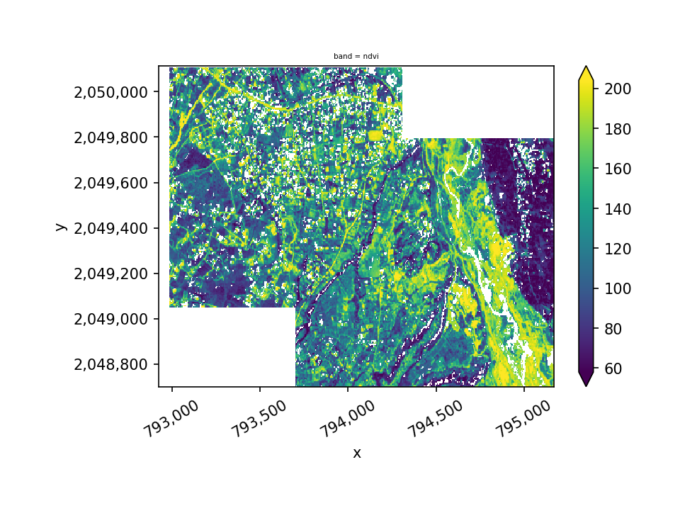
Masking With Another Raster

Geowombat also makes masking out values easy. To set a global mask follow this general proceedure.

NOTE: Masking can also be done using shapefiles, see mask.

with gw.config.update(sensor='bgrn', scale_factor=0.0001):
    with gw.open([rgbn_suba, rgbn_subb],
              mosaic=True,
              bounds_by='union') as ds_mos:
     print(ds_mos)

<xarray.DataArray (band: 4, y: 283, x: 449)>
dask.array<maximum, shape=(4, 283, 449), dtype=uint8, chunksize=(1, 64, 64), chunktype=numpy.ndarray>
Coordinates:
  * band     (band) <U5 'blue' 'green' 'red' 'nir'
  * y        (y) float64 2.05e+06 2.05e+06 2.05e+06 ... 2.049e+06 2.049e+06
  * x        (x) float64 7.929e+05 7.929e+05 7.929e+05 ... 7.952e+05 7.952e+05
Attributes:
    transform:   (5.0, 0.0, 792925.0, 0.0, -5.0, 2050115.0)
    crs:         +init=epsg:32618
    res:         (5.0, 5.0)
    is_tiled:    0
    nodatavals:  (0.0, 0.0, 0.0, 0.0)
    scales:      (1.0, 1.0, 1.0, 1.0)
    offsets:     (0.0, 0.0, 0.0, 0.0)
    sensor:      blue, green, red, and NIR
    resampling:  nearest

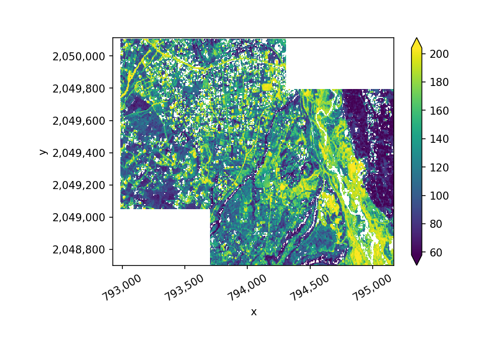
Masking can simply be accomplished with .where

masked = ds_mos.sel(band='blue').where(ndvi >= -0.25)
masked.sel(band='ndvi').gw.imshow(robust=True)

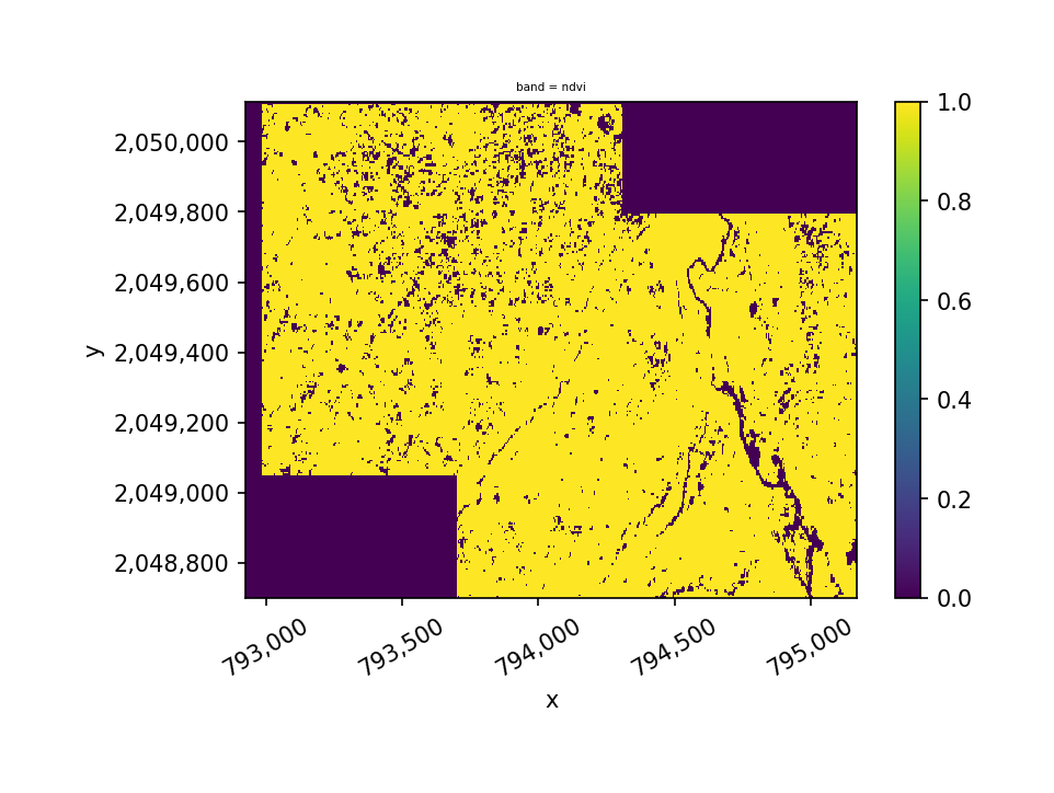
Storing a mask for later use

We can also create a masking layer that be be concatenated into the dataset for later use.

masker =  ndvi >= -0.25
masker.sel(band='ndvi').gw.imshow(robust=True)

ndvi_mask = ndvi*masker
ndvi_mask.sel(band='ndvi').gw.imshow(robust=True)

We can keep the mask as a separate array entity, or, if we are using it routinely, there are advantages to adding it as a band in the DataArray:

import xarray as xr
ds_mos_ndvi = xr.concat([ds_mos,masker], dim="band")
ds_mos_ndvi

<xarray.DataArray (band: 5, y: 283, x: 449)>
dask.array<concatenate, shape=(5, 283, 449), dtype=uint8, chunksize=(1, 64, 64), chunktype=numpy.ndarray>
Coordinates:
  * y        (y) float64 2.05e+06 2.05e+06 2.05e+06 ... 2.049e+06 2.049e+06
  * x        (x) float64 7.929e+05 7.929e+05 7.929e+05 ... 7.952e+05 7.952e+05
  * band     (band) object 'blue' 'green' 'red' 'nir' 'ndvi'
Attributes:
    transform:   (5.0, 0.0, 792925.0, 0.0, -5.0, 2050115.0)
    crs:         +init=epsg:32618
    res:         (5.0, 5.0)
    is_tiled:    0
    nodatavals:  (0.0, 0.0, 0.0, 0.0)
    scales:      (1.0, 1.0, 1.0, 1.0)
    offsets:     (0.0, 0.0, 0.0, 0.0)
    sensor:      blue, green, red, and NIR
    resampling:  nearest

ds_mos_ndvi.sel(band='blue').where(ds_mos_ndvi.sel(band='ndvi') == 1).gw.imshow(robust=True)

We can also apply a mask across multiple bands as follows:

ds_mos_ndvi.sel(band=['blue', 'green', 'red']).where(ds_mos_ndvi.sel(band='ndvi') == 1).gw.imshow(robust=True)