Moving windows

Moving window (focal) operations apply a statistic within a sliding neighborhood around each pixel. This is useful for smoothing, texture analysis, and edge detection on raster data.

src.gw.moving() supports the following statistics: 'mean', 'std', 'var', 'min', 'max', 'perc'. Window sizes must be odd integers (3, 5, 7, 11, …). Each band is processed independently.

See the geowombat.moving() API reference and the notebooks/moving_windows.ipynb notebook for interactive examples.

Setup

All examples below use the bundled Landsat 8 test image, subset to a small region with gw.config.update(ref_bounds=...) for speed and better visualization.

import geowombat as gw
from geowombat.data import l8_224078_20200518
import matplotlib.pyplot as plt

# Small subset in the upper-left of the image (EPSG:32621)
BOUNDS = (717345, -2783000, 723345, -2777000)

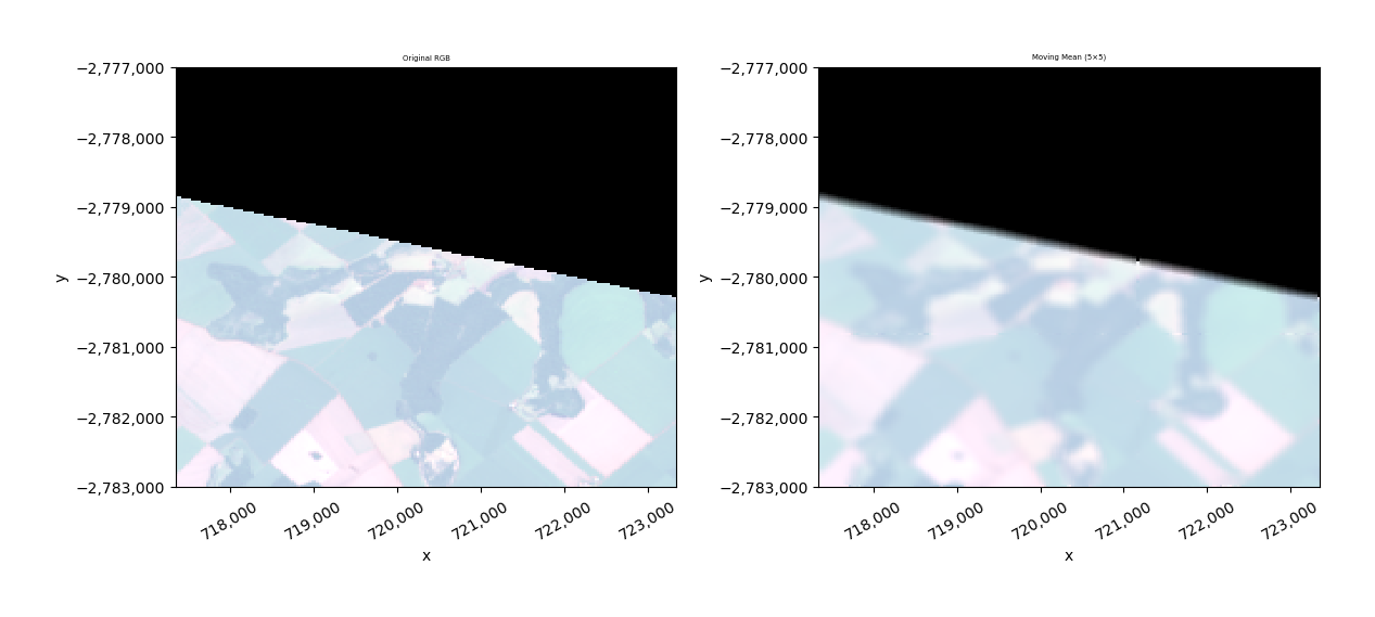
Basic usage: moving mean

Average pixel values within a 5x5 neighborhood. Set nodata=0 to exclude zero-valued pixels from the computation. Use .where(src != 0) to mask the nodata region in the result.

with gw.config.update(ref_bounds=BOUNDS):
    with gw.open(l8_224078_20200518, chunks=128, nodata=0) as src:
        result_mean = src.gw.moving(stat='mean', w=5, nodata=0)
        result_mean = result_mean.where(src != 0)

        fig, axes = plt.subplots(1, 2, figsize=(12, 5))
        src.sel(band=[3, 2, 1]).gw.imshow(
            mask=True, nodata=0, robust=True, ax=axes[0]
        )
        axes[0].set_title('Original RGB')
        result_mean.sel(band=[3, 2, 1]).gw.imshow(
            mask=True, nodata=0, robust=True, ax=axes[1]
        )
        axes[1].set_title('Moving Mean (5x5)')
        plt.tight_layout()
        plt.show()

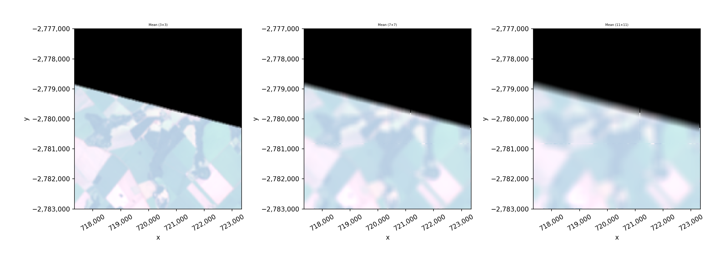
Comparing window sizes

Larger windows produce stronger smoothing.

with gw.config.update(ref_bounds=BOUNDS):
    with gw.open(l8_224078_20200518, chunks=128, nodata=0) as src:
        sizes = [3, 7, 11]
        fig, axes = plt.subplots(1, 3, figsize=(15, 5))

        for ax, w in zip(axes, sizes):
            result = src.gw.moving(stat='mean', w=w, nodata=0)
            result = result.where(src != 0)
            result.sel(band=[3, 2, 1]).gw.imshow(
                mask=True, nodata=0, robust=True, ax=ax
            )
            ax.set_title(f'Mean ({w}x{w})')

        plt.tight_layout()
        plt.show()

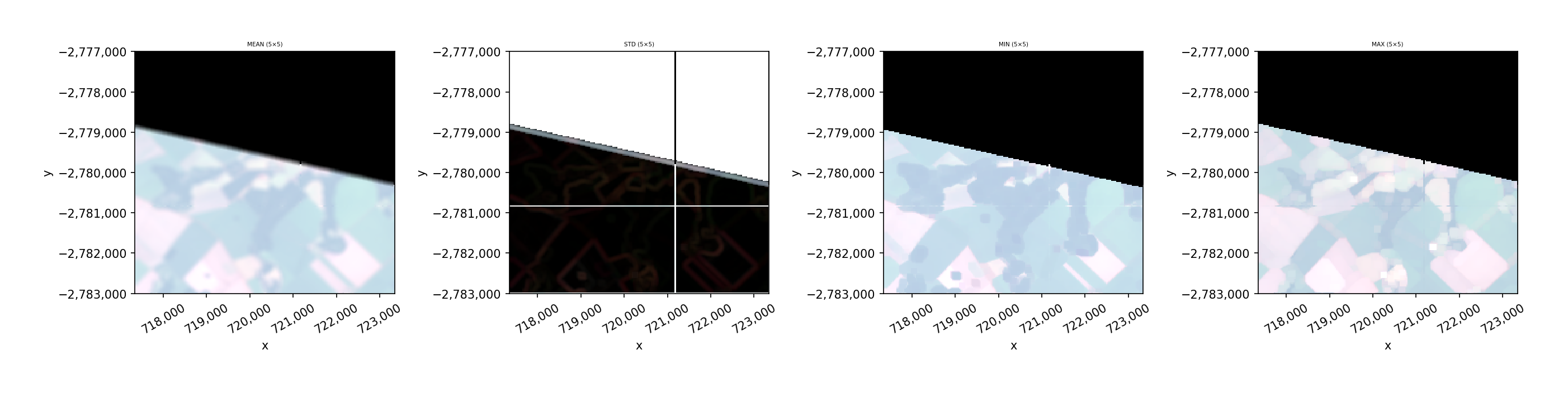
Different statistics

Beyond the mean, compute standard deviation (texture), min/max (morphological-style operations), and variance within the window.

with gw.config.update(ref_bounds=BOUNDS):
    with gw.open(l8_224078_20200518, chunks=128, nodata=0) as src:
        stats = ['mean', 'std', 'min', 'max']
        fig, axes = plt.subplots(1, 4, figsize=(18, 4))

        for ax, stat in zip(axes, stats):
            result = src.gw.moving(stat=stat, w=5, nodata=0)
            result = result.where(src != 0)
            result.sel(band=[3, 2, 1]).gw.imshow(
                mask=True, nodata=0, robust=True, ax=ax
            )
            ax.set_title(f'{stat.upper()} (5x5)')

        plt.tight_layout()
        plt.show()

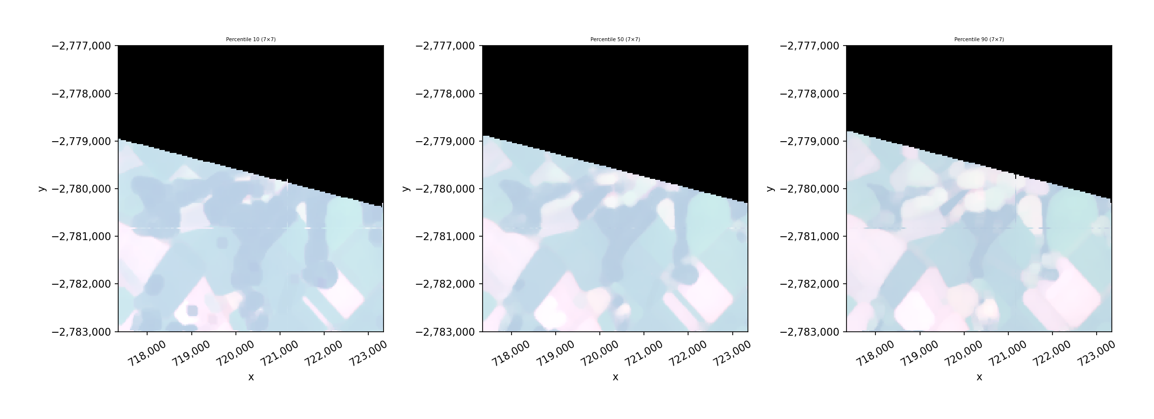
Percentile filter

Use stat='perc' with the perc parameter to compute a specific percentile within the window. This is useful for robust smoothing (e.g., median with perc=50) or highlighting bright/dark features.

with gw.config.update(ref_bounds=BOUNDS):
    with gw.open(l8_224078_20200518, chunks=128, nodata=0) as src:
        percentiles = [10, 50, 90]
        fig, axes = plt.subplots(1, 3, figsize=(15, 5))

        for ax, perc in zip(axes, percentiles):
            result = src.gw.moving(
                stat='perc', perc=perc, w=7, nodata=0
            )
            result = result.where(src != 0)
            result.sel(band=[3, 2, 1]).gw.imshow(
                mask=True, nodata=0, robust=True, ax=ax
            )
            ax.set_title(f'Percentile {perc} (7x7)')

        plt.tight_layout()
        plt.show()

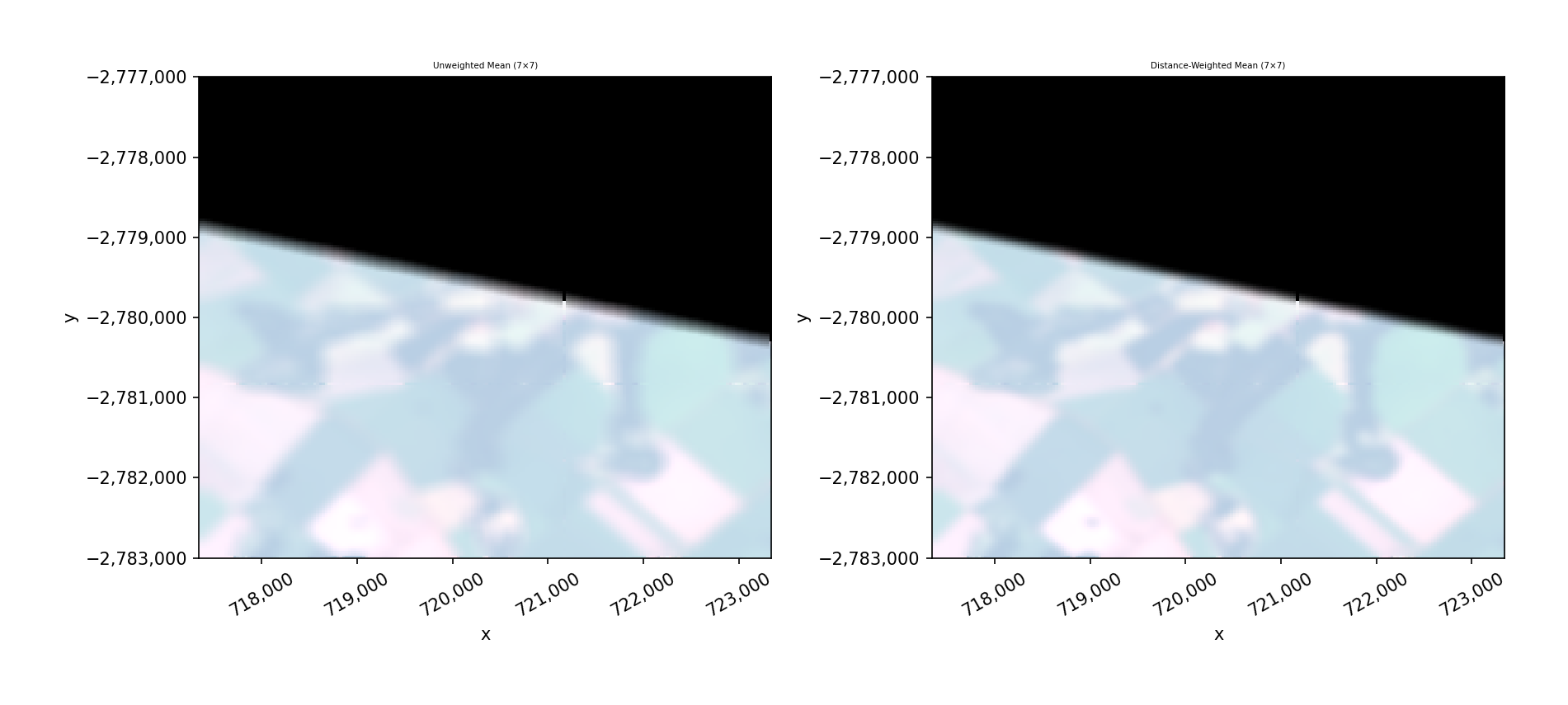
Distance-weighted moving window

Setting weights=True weights each pixel by its distance from the window center, giving more influence to nearby pixels. This produces a smoother result similar to a Gaussian-like filter.

with gw.config.update(ref_bounds=BOUNDS):
    with gw.open(l8_224078_20200518, chunks=128, nodata=0) as src:
        result_unweighted = src.gw.moving(
            stat='mean', w=7, nodata=0
        )
        result_unweighted = result_unweighted.where(src != 0)
        result_weighted = src.gw.moving(
            stat='mean', w=7, nodata=0, weights=True
        )
        result_weighted = result_weighted.where(src != 0)

        fig, axes = plt.subplots(1, 2, figsize=(12, 5))
        result_unweighted.sel(band=[3, 2, 1]).gw.imshow(
            mask=True, nodata=0, robust=True, ax=axes[0]
        )
        axes[0].set_title('Unweighted Mean (7x7)')
        result_weighted.sel(band=[3, 2, 1]).gw.imshow(
            mask=True, nodata=0, robust=True, ax=axes[1]
        )
        axes[1].set_title('Distance-Weighted Mean (7x7)')
        plt.tight_layout()
        plt.show()

Saving results

Moving window results are lazy dask arrays. Use .gw.save() to write to disk or .compute() to load into memory.

with gw.config.update(ref_bounds=BOUNDS):
    with gw.open(l8_224078_20200518, chunks=128) as src:
        result = src.gw.moving(stat='mean', w=5, nodata=0)

        # Compute into memory
        result_computed = result.compute()

        # Save to file
        result.gw.save('smoothed_output.tif', overwrite=True)

Notes

• Nodata handling: Pass nodata=0 (or your nodata value) to moving() so those pixels are excluded from the window computation. Then mask the result with .where(src != 0) to set nodata regions to NaN for display and downstream analysis.

• Window size must be an odd integer. Even values raise an error.

• Multi-band: Each band is processed independently. The result has the same shape as the input.

• Chunks: Moving windows use dask map_overlap with reflected boundaries. Chunk borders are handled transparently.